|
By Avery Hinks Often in the field of biomechanics and muscle physiology, we construct graphs of the relationship between one muscle variable and another. For example: the relationship between muscle length and muscle force (the active force-length relationship), the relationship between force and the concentration of calcium in a muscle fibre (the force-pCA relationship), or the relationship between muscle force and contraction speed (the force-velocity relationship). 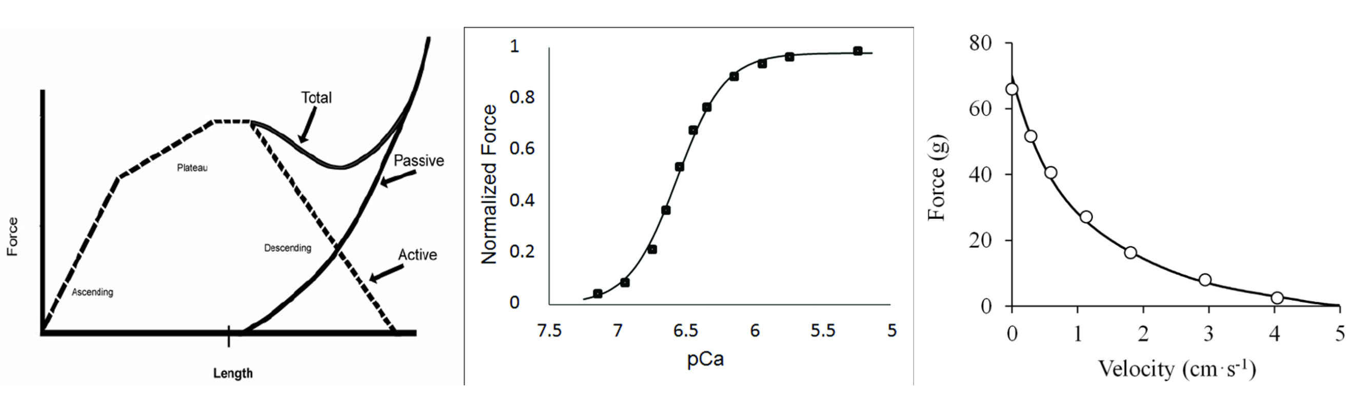 Graphs from: Knudson (2006), Journal of Exercise Science and Physiotherapy; Zhang et al. (2018), Frontiers in Physiology; Alcazar et al. (2019), Frontiers of Physiology. After constructing these relationships from collected data, the question often arises of how to display these data across multiple participants, and make comparisons between groups. For example, a group that completed a training program versus a group that didn’t, or a group of younger versus older individuals. Graphing each collected data point can make statistical analyses difficult. To get around this, many often fit the data to an equation. Fitting data to an equation allows the generation of infinite theoretical data points based on the trends within your data, and the comparison of constants between participants and groups. A prominent example, and the example I will be using throughout this knowledge translation, is the force-velocity relationship. The force-velocity relationship is often fitted to the following equation developed by Hill (1938): 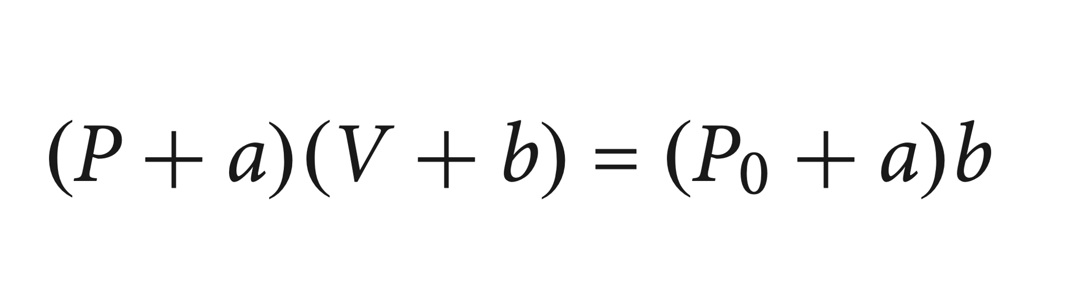 In the equation above, P represents force and V represents velocity. a and b are adjustable constants, with a representing the heat produced during shortening and b representing the increase in energy as force decreases. The first time someone suggested I fit my data to an equation, I was horrified. I’d heard too many stories of people spending hours in coding software such as R or Python. But have no fear! Fitting data to an equation can be easier than it’s made out to be, and you can do it accurately in Excel. Today, I’m going to show you how that works. First, let’s talk about the Force-Velocity RelationshipTo generate strength in muscle, many small proteins called actin and myosin bind to form “cross-bridges”. The formation of these cross-bridges produces force, and that’s what gives our muscle the strength to push, pull, walk, and run.  When lifting an object, muscle undergoes a “concentric” contraction, which means it shortens while producing force.  When a muscle shortens very slow, actin and myosin can easily bind each other, leading to near-maximal force production. However, as the muscle shortens faster, more of these actin and myosin filaments slide past each other without the opportunity to bind. Therefore, the ability for muscle to produce force decreases with increasing shortening velocity. From this principle, the force-velocity relationship looks like this: 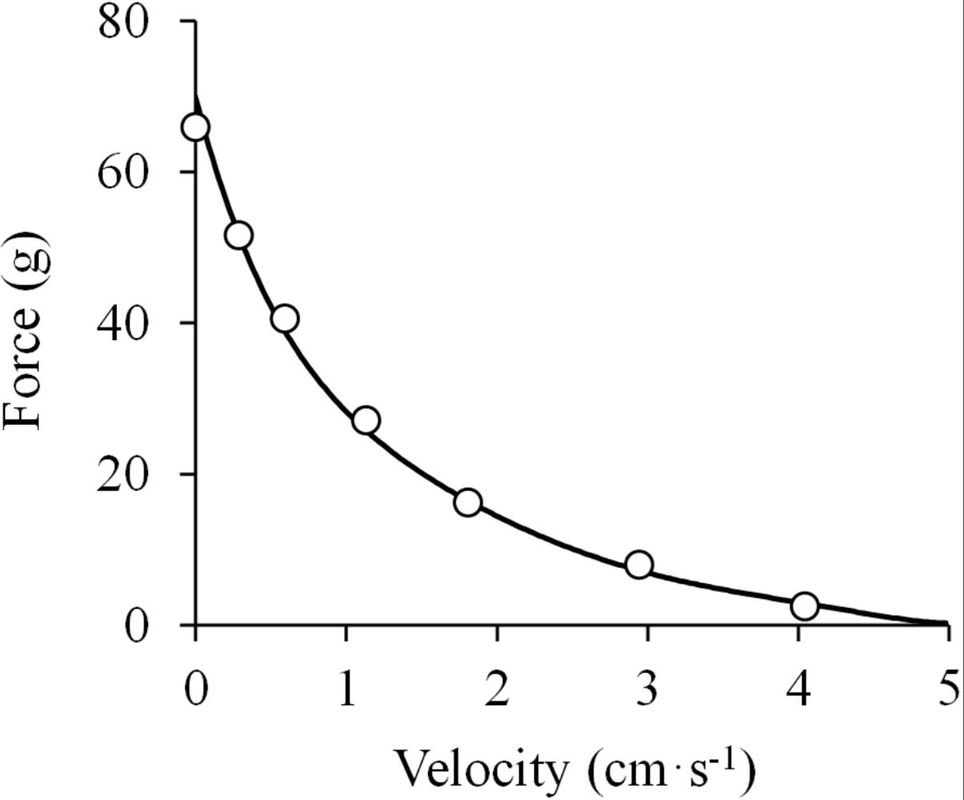 From Alcazar et al. (2019), Frontiers of Physiology. In the graph above, the white circles represent the collected data points, and the line represents the curve generated from fitting the points to Hill’s equation. I have my data points. Now what do I do?After collecting data for muscle shortening velocity across various levels of force, you’re ready to fit them to an equation! I will go through the Excel method step by step. First, make sure you have the “Solver” add-on in Excel turned on. To do this, first click on the “Data” tab.  In the Data tab, all the way to the right, click “Analysis Tools”.  An “Add-ins” pop-up will appear. Check “Solver Add-In” then click “OK”.  You should now see the “Solver” tool in your Data tab.  Now you can get started! The data I’ll be using as an example is from one of the first force-velocity papers, by A.V. Hill in 1938. 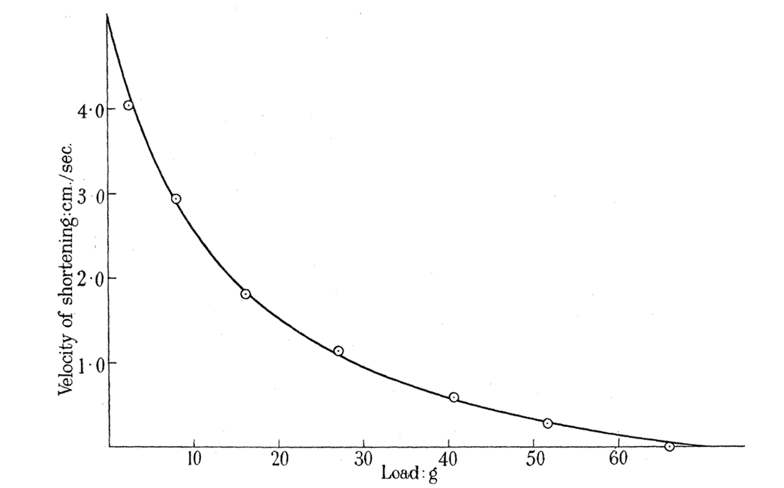 First, you’ll want to make the following column labels: 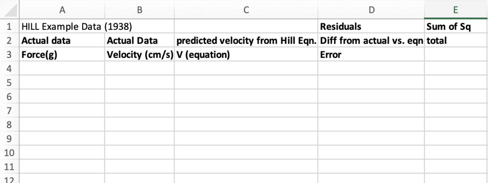 Next, fill in the first two columns with the Force and Velocity data you collected. Additionally, add a box showing the mean (average) velocity value, which will be important later. 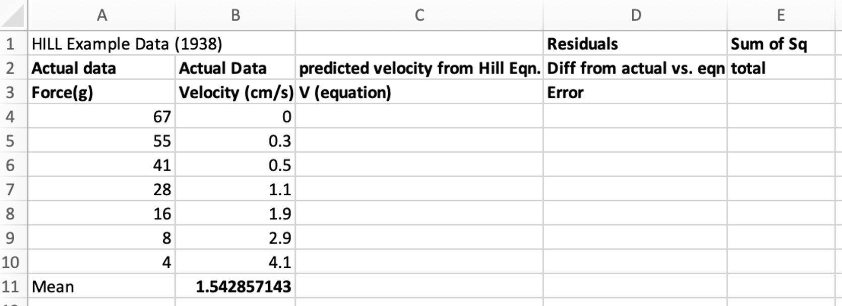 Now we look to Hill (1938)’s equation: We want to use this equation to calculate velocities from given force values. Therefore, before we do anything else, we need to re-arrange this equation to isolate V. If you’ve blocked out everything you learned in 12th grade algebra, do not worry. Here are the steps: (P + a) (V + b) = (Po + a) b If we divide both sides by (P + a), we have: V + b = ((Po + a) b) / (P + a) Now we just have to subtract b from both sides: V = (((Po + a) b) / (P + a)) – b This is the equation we’ll be using for our curve fitting! As a reminder: in this equation, V is the calculated velocity, P is a given force value, Po is the maximum force (i.e., force at 0 velocity), and a and b are adjustable constants. What we want to do with our solver is adjust a and b so that the calculated velocities fit our collected data as best as possible. To do this, we first need to add cells for a, b, and Po. 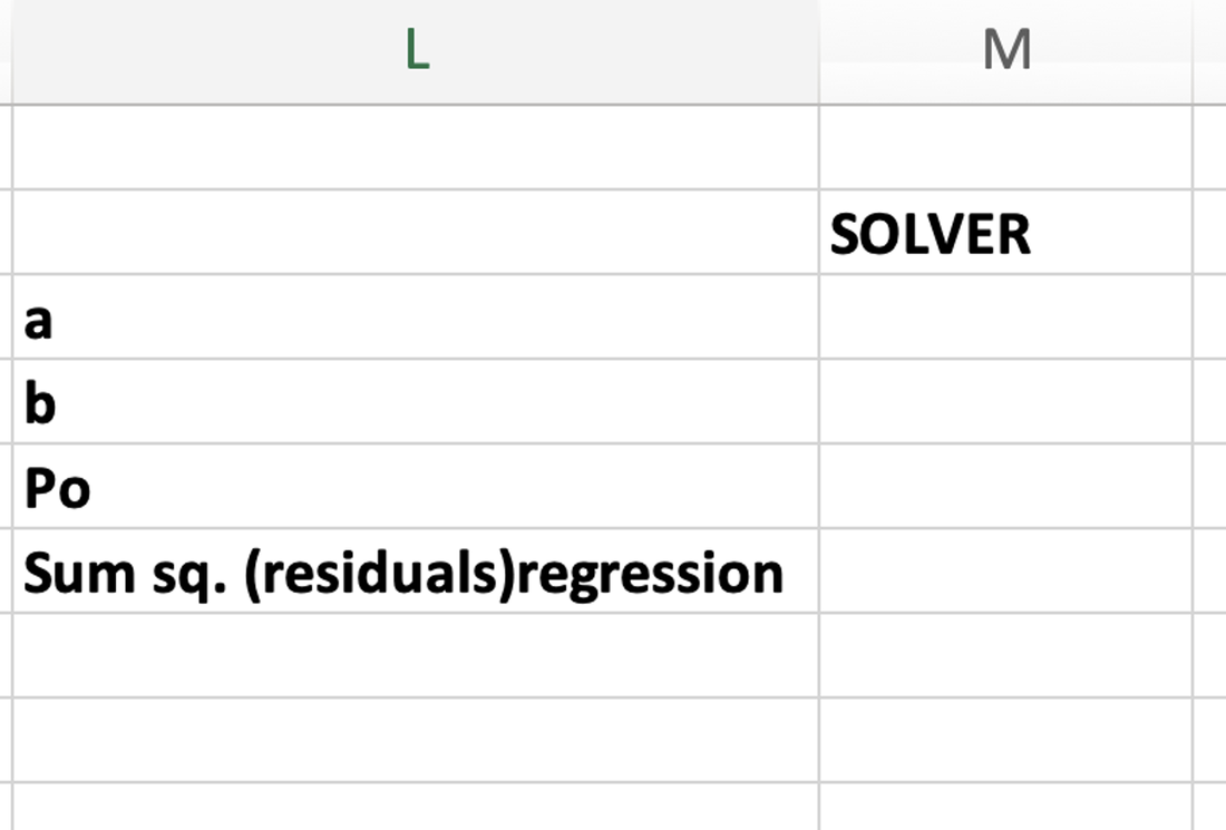 The “Sum sq” cell will come in handy in a moment, too. I recommend placing these cells at about this distance (see below) from the columns we made earlier. You’ll see why over the next few steps. 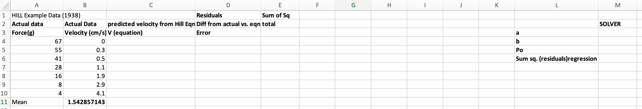 We can now fill the equation in the “Predicted Velocity” column as follows: 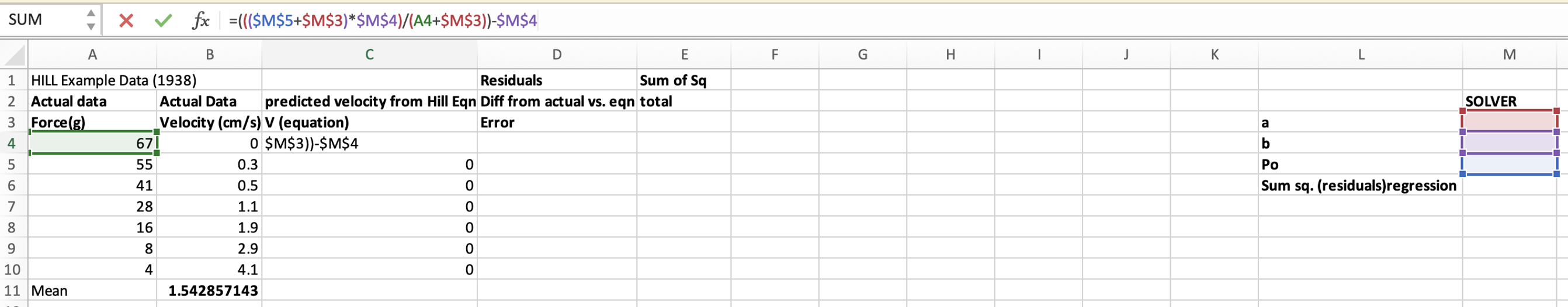 For now, because the constants are empty, all the values come up as 0. To best visualize the curve-fitting in action, we can construct a graph showing two separate plots: one with the collected velocity on the Y-axis and collected force on the X-axis; and one with the calculated velocity on the Y-axis and collected force on the X-axis. Since our predicted velocity column is not filled in yet, it will start out looking like this: 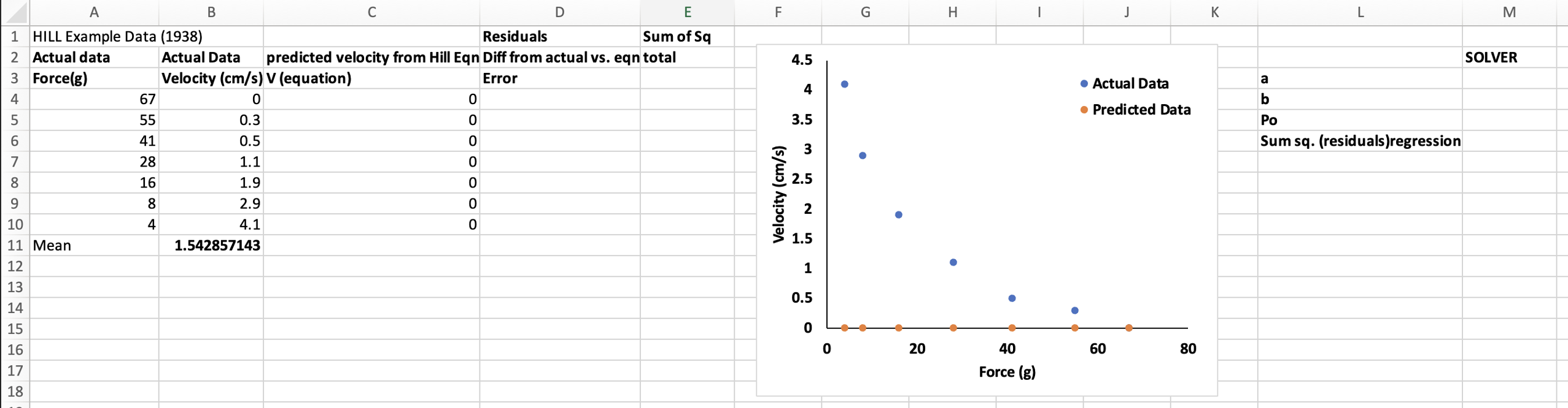 Now we’ll fill in the two remaining columns: “Error” and “Sum of Squares total”. In the Error column, we want the difference between the predicted and collected velocities, so we use the following equation: 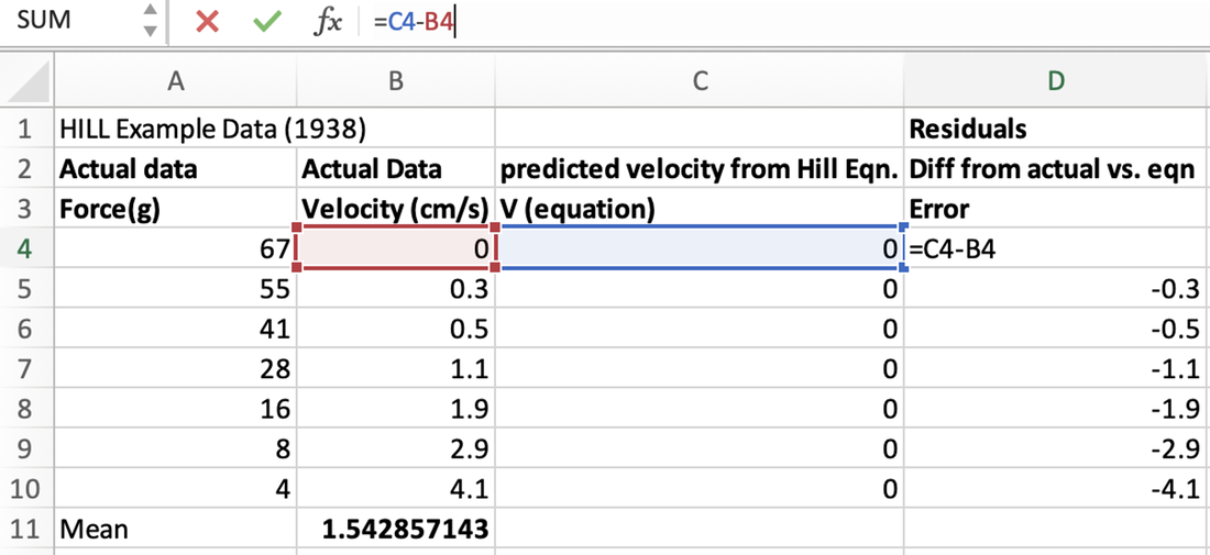 In the Sum of Squares Total column, we want the difference between each collected velocity data point and the mean collected velocity, so we use this equation: 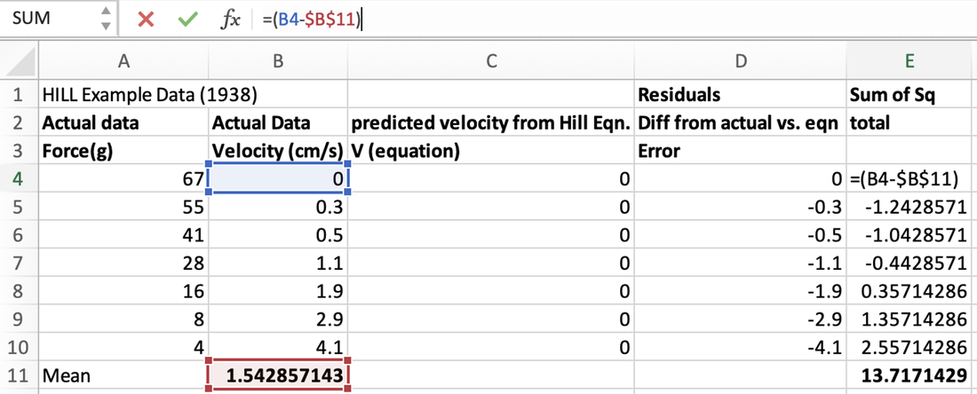 The bolded value below the Sum of Squares Total column is the Sum of Squares Total value. We compute this with the following equation: 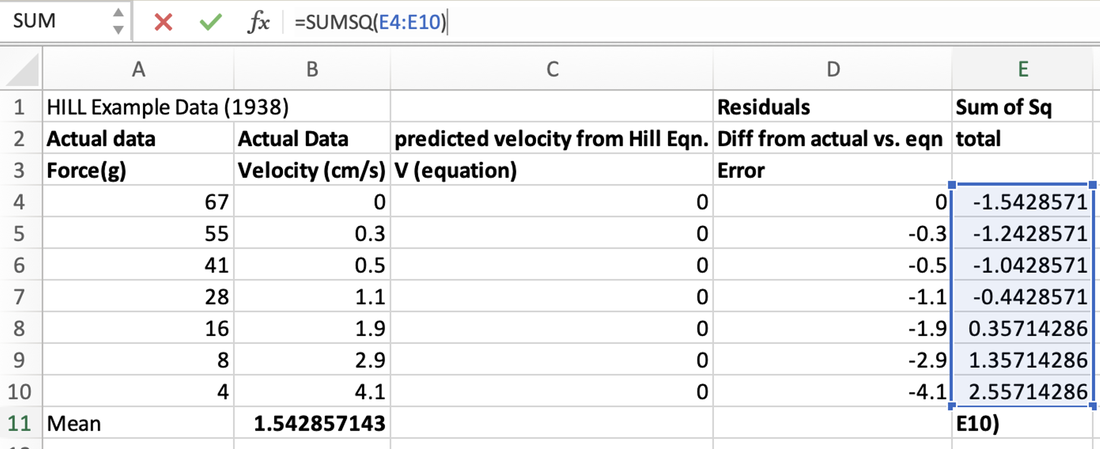 Now that our equations are all setup, we can fill in the constants. For Po, we can see that the maximum force is 67, so that’s what we put there. For a and b, the starting values are mostly arbitrary, but they have to be relatively close to the proper values. What do I mean by this? Basically, you can adjust a and b while watching the orange points on the graph until the trends made by both the orange and blue points are clearly visible. For example, here I’ve started a at 9 and b at 2: 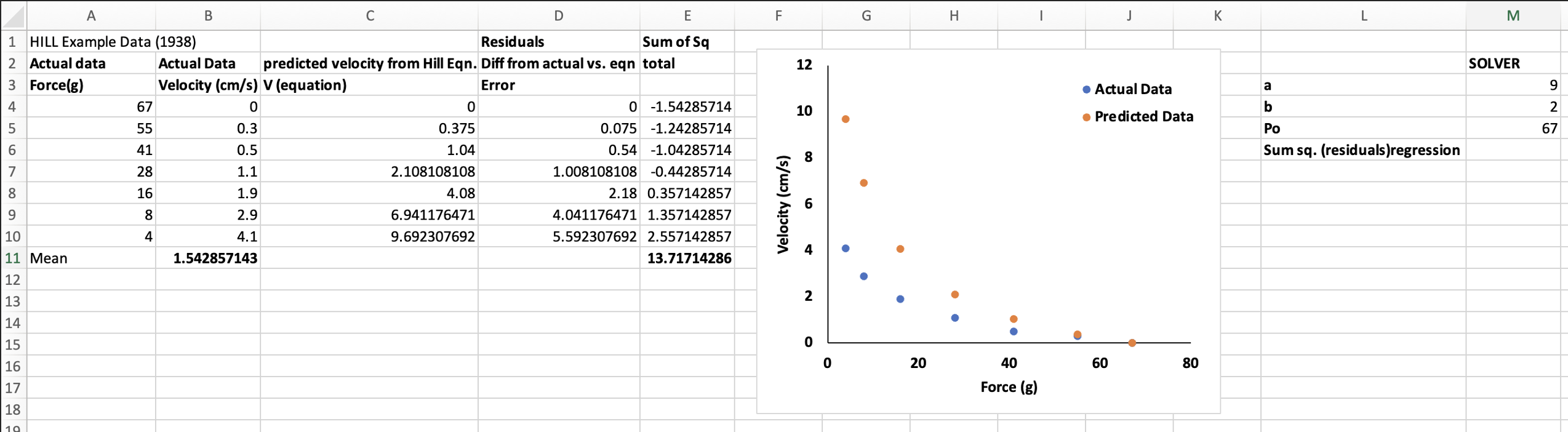 These should be close enough for the Solver to work with. One more step before I employ the Solver. We need to fill in the “Sum of squares residuals” box under Po. This value represents the Sum of Squares of the “Error” column and may be the most important value for the Solver. To compute this, we use the following equation: 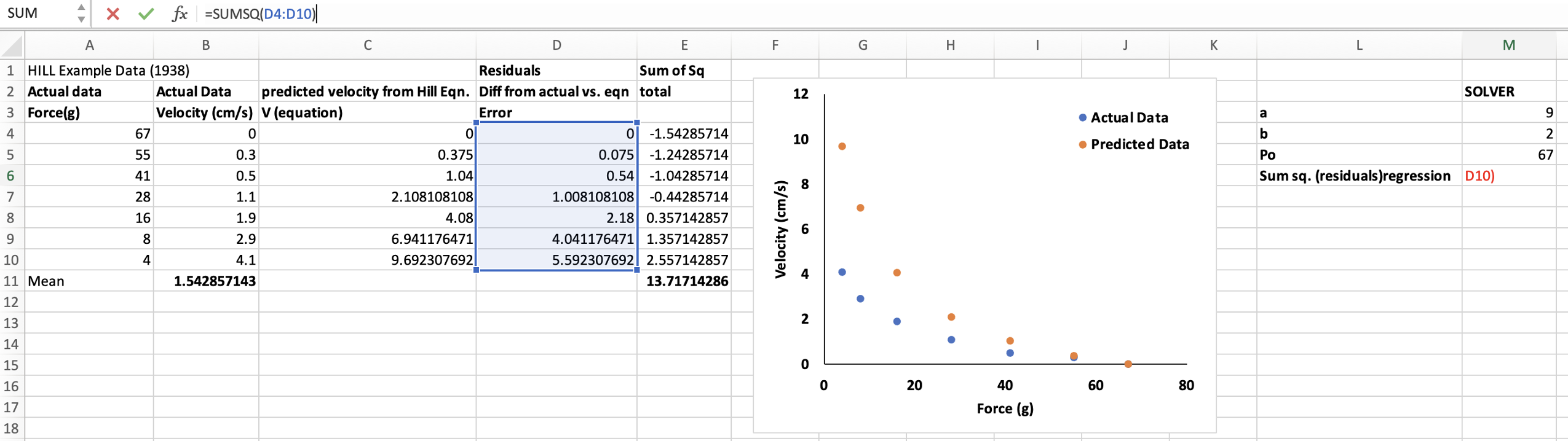 And we end up with a starting Sum of Squares Error of 53.67. This is a very high error value, and makes sense since the orange data points are currently far away from the blue data points. The Solver will work to minimize this Sum of Squares Error to make the predicted values as close as possible to the collected values. 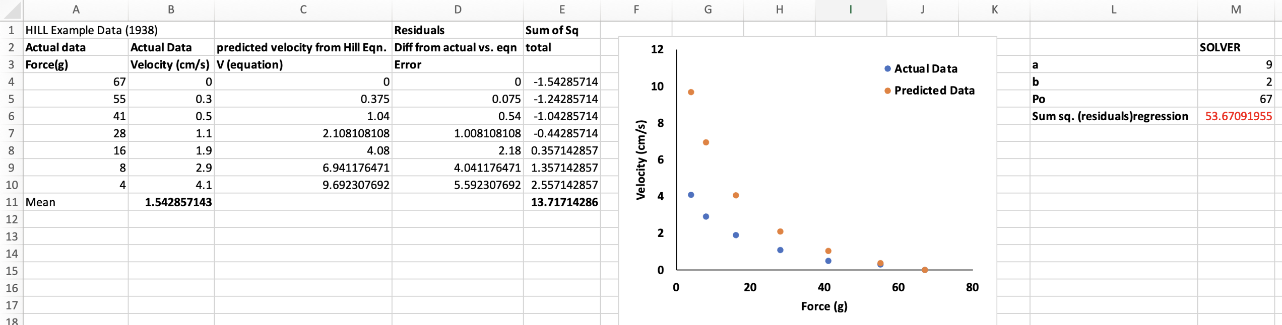 Now, go to the “Data” tab, and open the “Solver”. This window will pop up: 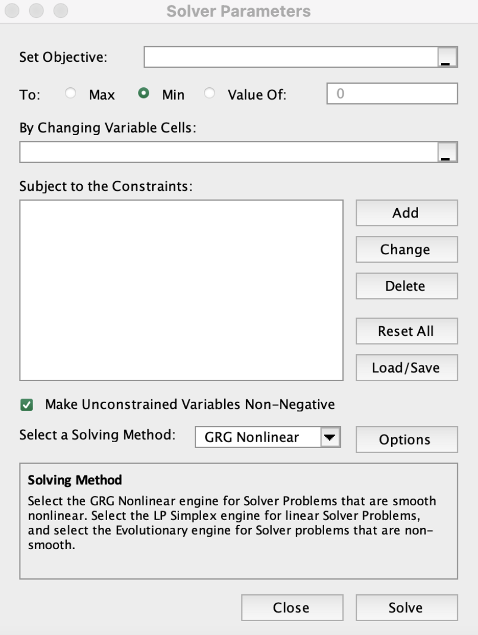 First, we want to set our objective. This will be the Sum of Squares Error cell. We also select “Min” because we want the Solver to minimize this error. 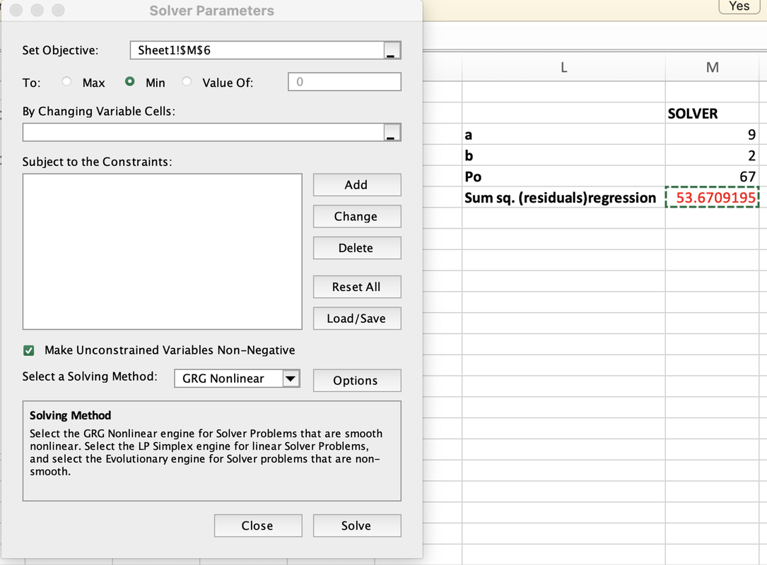 Under “By Changing Variable Cells”, we select the a and b constants, because we want the Solver to adjust these constants to minimize the error. 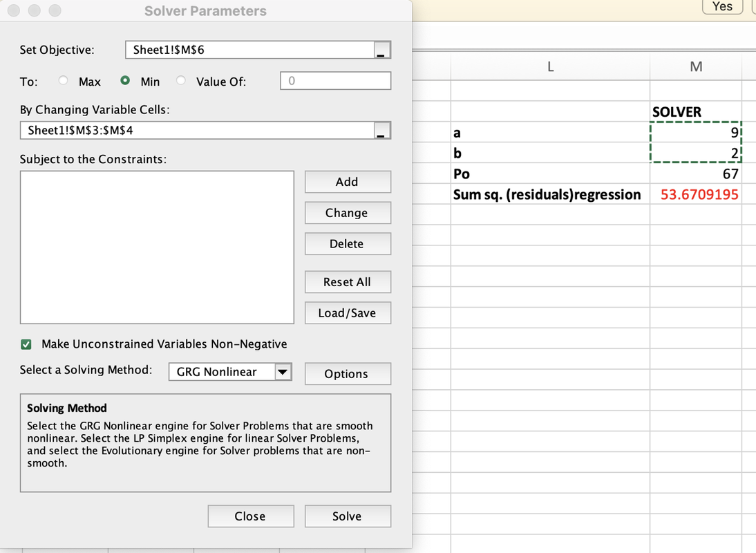 Now we click “Solve”! I’ve recorded a video so you can watch what the Solver looks like in real time: https://drive.google.com/file/d/1lbQQu3ttDt8et-kY8LFrV88GrydB1IIC/view?usp=sharing As you can see, once the Solver is done, a and b have been determined, the Sum of Squares Error has been minimized (from 53.67 to 0.04), and the orange dots fit the blue dots much better! 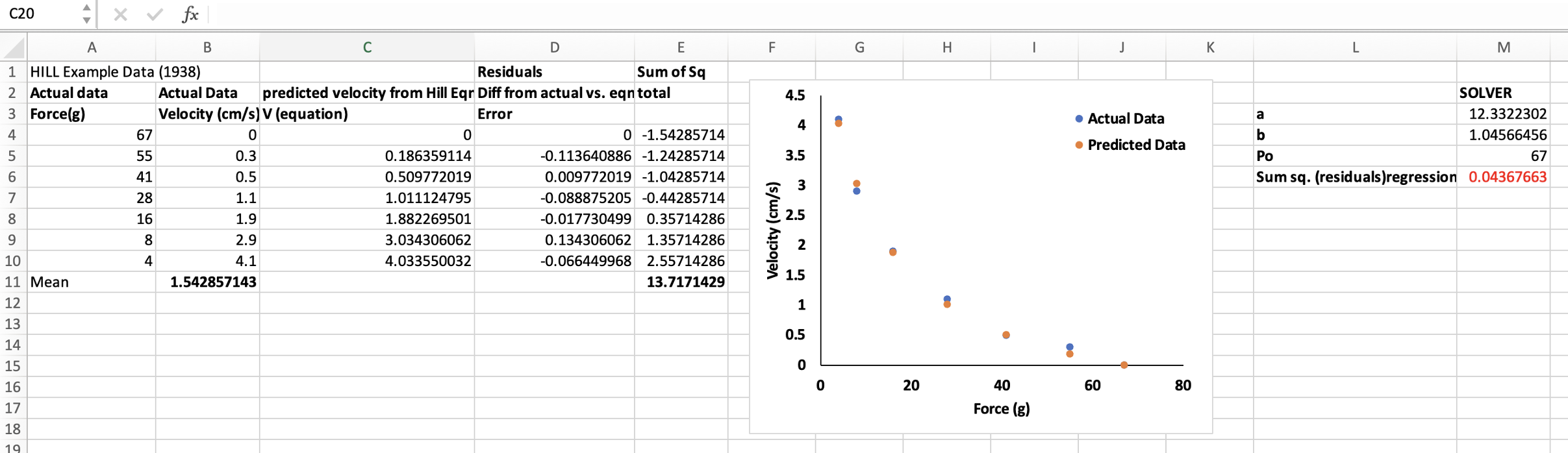 You probably noticed in the video that there are a few things I haven’t added in yet. The first is the R^2 value. This value will tell you how good of a fit your Solved data points are to your collected data points. The maximum R^2 value is 1.0 (meaning a 100% fit), and generally we want at least 0.98 as indication of a good fit. To calculate R^2, we will divide the Sum of Squares Residuals by the Sum of Squares Total, then subtract the result from 1. In Excel, we use this equation:  For this example, we end up with an R^2 of over 0.99, indicating our Solved force-velocity curve fits our data very well! 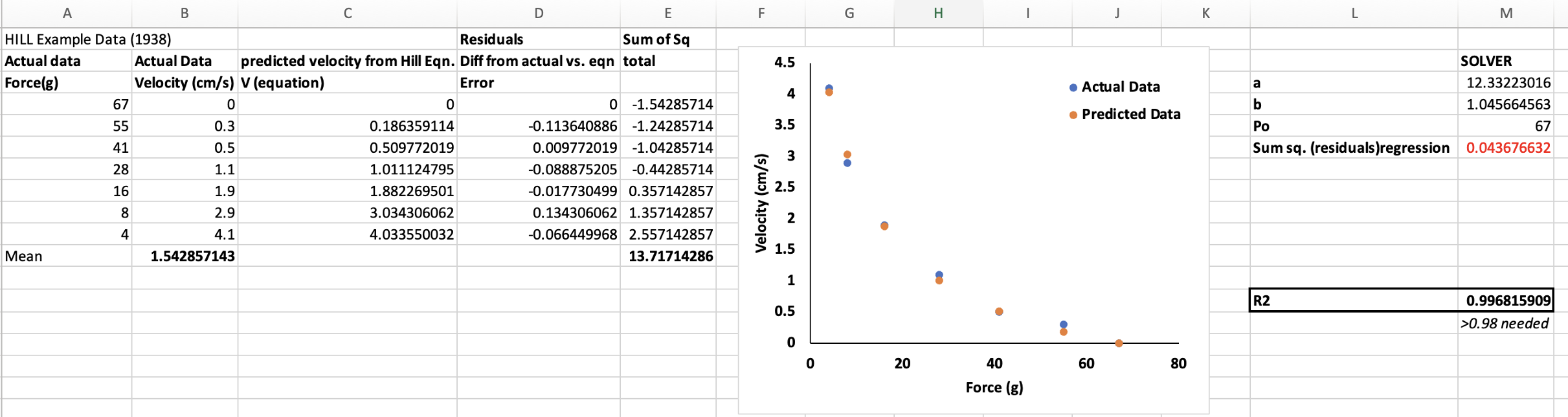 This Solver has ultimately given us values to fill in our original Hill (1938) equation: V = (((67 + 12.33223) 1.04566) / (P + 12.33223)) – 1.04566 From this, we can calculate velocity across an infinite number of force data points, and end up with a very clean force-velocity curve. 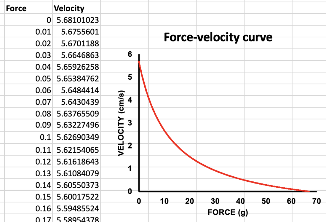 Plotting the data like this also allows us to obtain other key values associated with the force-velocity relationship. For example: the curvature of the force-velocity curve, which is equal to a divided by Po; and the maximum shortening velocity (Vmax), which is nearly impossible to obtain from real data collection. 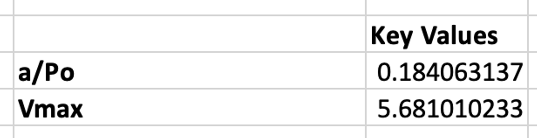 One of the best markers of dynamic muscle performance is power. Power is the product of force and velocity; therefore, we can obtain the maximum power (Pmax) from these data as well. 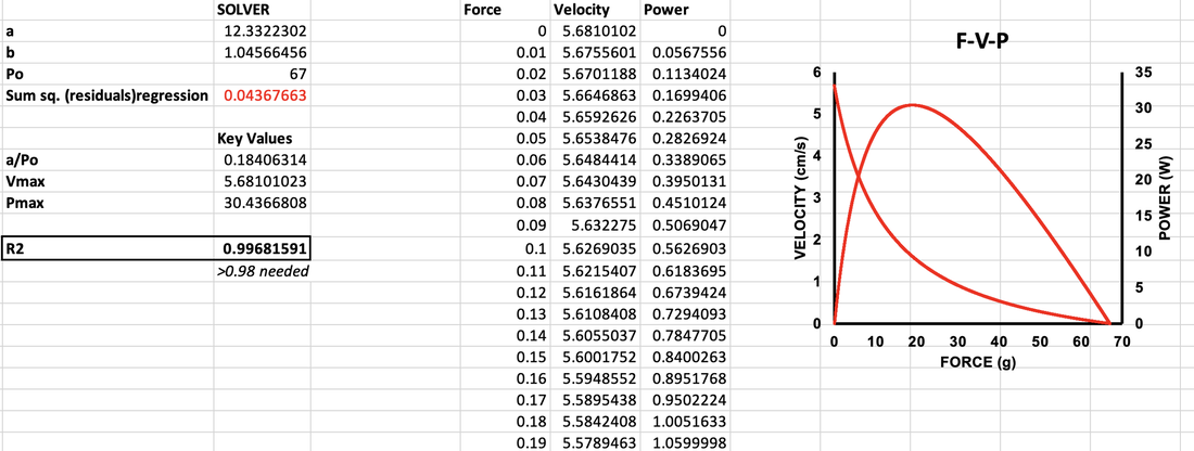 If this process is completed for each participant (whether the data is from a human performing voluntary contractions or a dissected mouse muscle), we can statistically compare the constants and these key values between different groups! For example, the study that produced the graph below compared the force-velocity relationship before (Pre) and after (Post) resistance training, and after a period of de-training (Post-Detr). 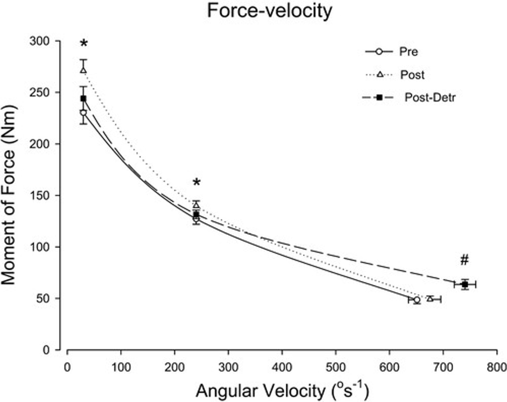 From Andersen et al. (2005), Journal of Applied Physiology. This curve-fitting method works for any equation, including equations with more constants than the force-velocity example I showed here. For example, in a paper by Mohammed and Hou (2015), they suggest using the following asymmetric Gaussian function for fitting the active force-length relationship: 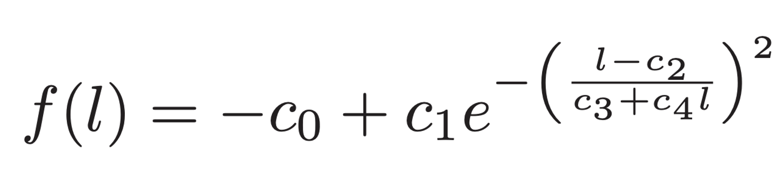 This equation has five constants to adjust for fitting a curve. I have previously used the Excel Solver add-on to fit active force-length data to this equation (see: Hinks et al., 2022, Biology Open), and it worked! Are there any disadvantages to curve-fitting?There are of course limitations to curve-fitting data. The most notable limitation is the accuracy of the equation you wish to use. Staying on the topic of the force-velocity curve, it has long been argued whether this relationship should be represented by a hyperbolic function (the equation used in my Excel example above) or a double-hyperbolic function, which is more intricate: 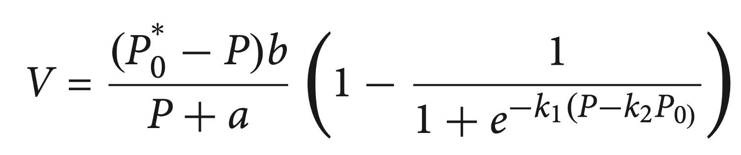 In 1976, Edman and colleagues challenged Hill’s original equation due to various observations over the years where force-velocity data could not be estimated by Hill’s equation. Edman’s findings argued that above 78% of maximum force, there is an inflection point. This inflection point appears to represent a transition toward the shape of the eccentric force-velocity relationship. For the eccentric force-velocity relationship, force is measured during lengthening (as opposed to concentric/shortening) contractions, and an increase in force with increasing lengthening velocity is observed. 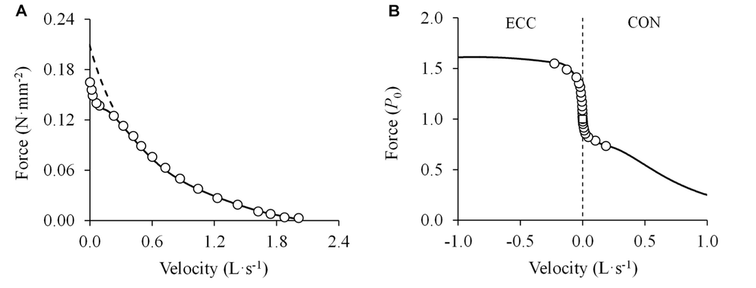 From Alcazar et al. (2019), Frontiers of Physiology. ‘A’ shows a double-hyperbolic force-velocity relationship collected from Edman’s experiments. ‘B’ demonstrates how this double-hyperbolic shape aligns with the shape of the eccentric (ECC) force-velocity relationship. Whether you should employ Hill’s hyperbolic equation or Edman’s double-hyperbolic equation in your curve-fitting is up for debate, and depends on the nature of your experiments. For example, if your experiment incorporates assessment of both shortening and lengthening contractions, Edman’s method is likely better. Alternatively, if your experiment only involves shortening contractions, you could fit your data to both equations and see which produces greater R^2 values. For a more in-depth comparison between these two representations of the force-velocity relationship, look to the review in Frontiers of Physiology by Alcazar and colleagues (2019). Another potential disadvantage to curve-fitting is for some participants, you may end up with a less than ideal R^2 value (for example, 0.90). Here, you may have to decide whether or not to cut said data from your analyses, or at least determine criteria for the lowest R^2 value you will accept. Regardless, curve-fitting is an excellent method of seeing how your data stands among previous literature. For anyone interested, I have provided the Excel sheet for the force-velocity example presented here. If you’ve made it to the end of this knowledge translation piece, I wish you the best in your future curve-fitting endeavours!
References
Alcazar J, Csapo R, Ara I, Alegre LM. On the Shape of the Force-Velocity Relationship in Skeletal Muscles: The Linear, the Hyperbolic, and the Double-Hyperbolic. Front Physiol. 2019 Jun 19;10:769. doi: 10.3389/fphys.2019.00769. PMID: 31275173; PMCID: PMC6593051. Andersen LL, Andersen JL, Magnusson SP, Suetta C, Madsen JL, Christensen LR, Aagaard P. Changes in the human muscle force-velocity relationship in response to resistance training and subsequent detraining. J Appl Physiol (1985). 2005 Jul;99(1):87-94. doi: 10.1152/japplphysiol.00091.2005. Epub 2005 Feb 24. PMID: 15731398. Edman KA, Mulieri LA, Scubon-Mulieri B. Non-hyperbolic force-velocity relationship in single muscle fibres. Acta Physiol Scand. 1976 Oct;98(2):143-56. doi: 10.1111/j.1748-1716.1976.tb00234.x. PMID: 1086583. Hill, A. V. (1938). The heat of shortening and the dynamic constants of muscle. Proceedings of the Royal Society of London. Series B-Biological Sciences, 126(843), 136-195. Hinks A, Jacob K, Mashouri P, Medak KD, Franchi MV, Wright DC, Brown SHM, Power GA. Influence of weighted downhill running training on serial sarcomere number and work loop performance in the rat soleus. Biol Open. 2022 Jul 15;11(7):bio059491. doi: 10.1242/bio.059491. Epub 2022 Jul 25. PMID: 35876382; PMCID: PMC9346294. Knudson, D. (2006). The biomechanics of stretching. Journal of Exercise Science and Physiotherapy, 2, 3-12. Mohammed GA, Hou M. Optimization of Active Muscle Force-Length Models Using Least Squares Curve Fitting. IEEE Trans Biomed Eng. 2016 Mar;63(3):630-5. doi: 10.1109/TBME.2015.2467169. Epub 2015 Aug 11. PMID: 26276984. Zhang X, Liu ZQ, Campbell KS, Wenk JF. Evaluation of a Novel Finite Element Model of Active Contraction in the Heart. Front Physiol. 2018 Apr 23;9:425. doi: 10.3389/fphys.2018.00425. PMID: 29740338; PMCID: PMC5924776.
0 Comments
|
AuthorAvery Hinks Archives
September 2023
Categories |
||
 RSS Feed
