|
By Dr. Geoff Power  You may have heard the phrase ‘old man strength’ often used in the context of someone performing a physical task seemingly above the level of performance you would expect for their age. To describe this phenomenon, the urban dictionary has used phrasing such as “The uncanny ability of older men to lift copious amounts of lumber, heavy furniture and beat their sons in arm wrestling”. You may have even overheard or had similar conversations as: “My dad beat me in arm wrestling again”, - ‘of course, he has old man strength”. In this article I will highlight one aspect of the human neuromuscular system which seems to resist the deleterious effects of age, the age-related maintenance of eccentric strength. 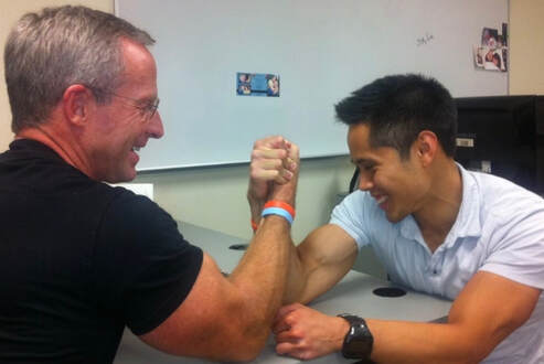 On one hand, natural adult aging is associated with many ‘negative’ alterations to the neuromuscular system resulting in muscle weakness and impaired functional performance of everyday tasks. Some of these changes include a loss of muscle mass through the death and dysfunctional remodelling of motor units (the basic ‘functional’ contractile unit consisting of the motor neuron housed in the spinal cord and its associated muscle fibres). 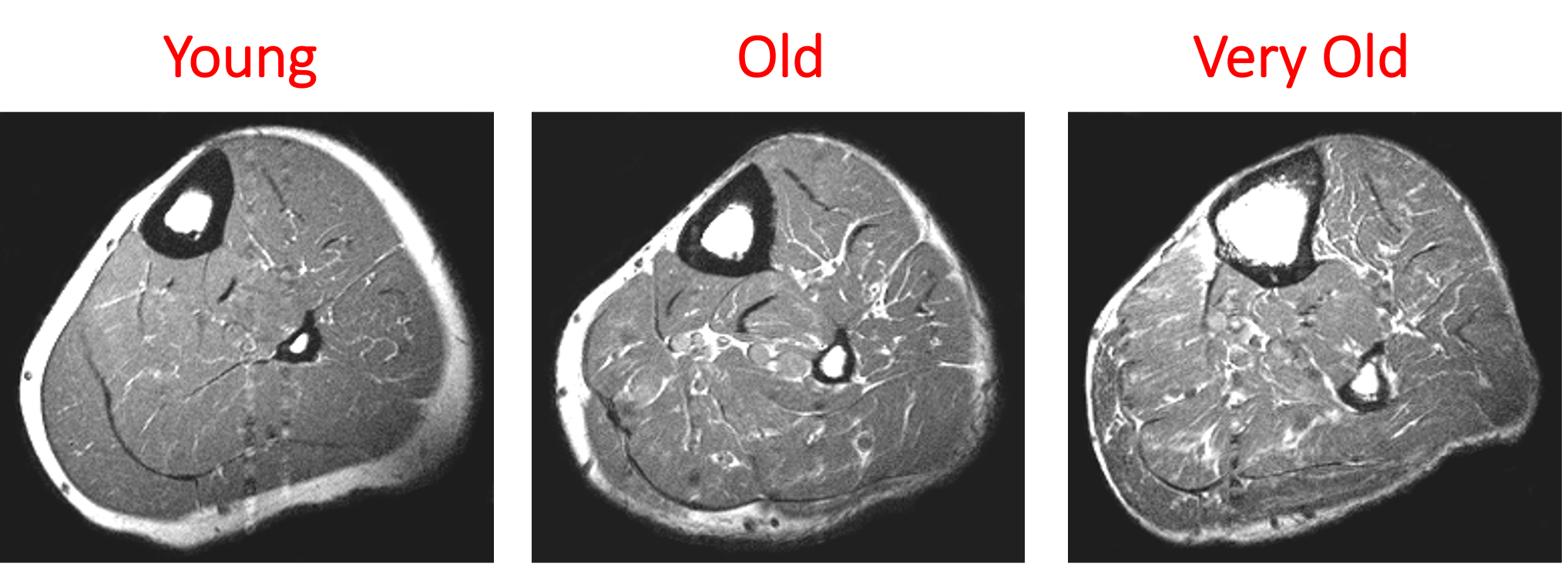 Figure: From youth to old age, there is a loss of contractile muscle tissue, and infiltration of fat and non-contractile tissue contributing to muscle weakness and impairments in muscle performance. A reduced ability to activate the remaining muscle mass through a reduction in the fidelity of the neural signals from the from the brain to the muscle. As well, owing to reductions in strength and speed of muscle contraction, power is drastically impaired. Importantly, it is power that is critical to performing daily tasks such as rising from a chair or walking up a flight of stairs. 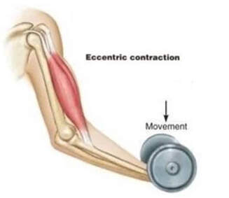 On the other hand, while many of the ‘negative alterations’ to the aging neuromuscular system are evident during static or shortening muscle actions, during lengthening actions (see our previous Knowledge Translation), performance is well-maintained to that of younger adults. A lengthening muscle action (or eccentric contraction) is unique in that the muscle generates an internal tension which is less than the external load, thus the muscle actively lengthens. Eccentric contractions are part of everyday movements such as walking down a flight of stairs, and older adults have elevated performance (relative to other contraction modes) and in some instances equal that of a healthy young adult. 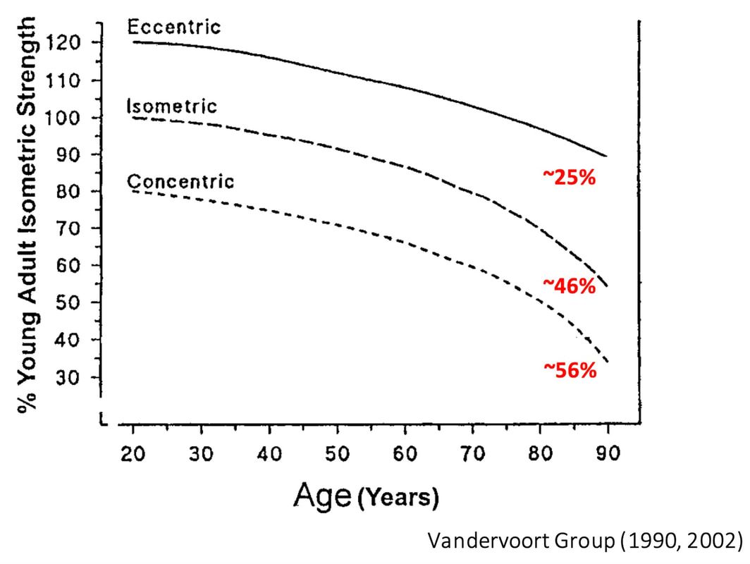 Figure: The above graph shows the age-related loss of strength during 3 distinct contraction types relative to a young adult: Static (isometric), shortening (concentric), and lengthening (eccentric). The largest deficits occur over time for the shortening contractions, which is a proxy of power. Static contractions show a similar but less drastic decline, and Eccentric contraction strength is well-maintained far into old age. Some of the suggested mechanisms contributing to a maintenance of eccentric strength in old age include: 1) An increase in non-contractile tissue infiltration such as collagen content/cross-linking. This means less contractile tissue is contributing to force during static and shortening contractions, impairing performance when the muscle is responsible for generating tension. However, more structures now ‘resist’ the external load during the lengthening (eccentric) contraction, increasing performance. The elevated passive stiffness of muscle in old age could also increase the effective ‘storage’ of elastic energy to optimize force production. 2) Eccentric contractions require less voluntary neural activation, meaning there is less of an impairment during lengthening contractions compared to static and shortening contractions. 3) There is an overall slowing of cross-bridge kinetics and increased proportion of weakly bound cross-bridges in old compared to young muscle. As active force generation depends on the number of strongly bound cross-bridges, any reduction or weakening of these cross-bridges will lessen active force generation. However, when external tension is applied, as in the case of a lengthening contraction, this cross-bridge configuration is optimized to resist active lengthening, and generate high forces. Work from our lab investigated the effects of slowing muscle cross-bridge kinetics, and biasing the cross-bridge configuration to more weakly bound states on the age-related maintenance of eccentric strength. We found that we could make young muscle act like old muscle when the muscle temperature was reduced to cause a slowing of muscle contraction. Therefore, if we look to interventions to reverse some of the age-related slowing of muscle contractile properties, we may identify strategies to improve power and performance during activates of daily living. 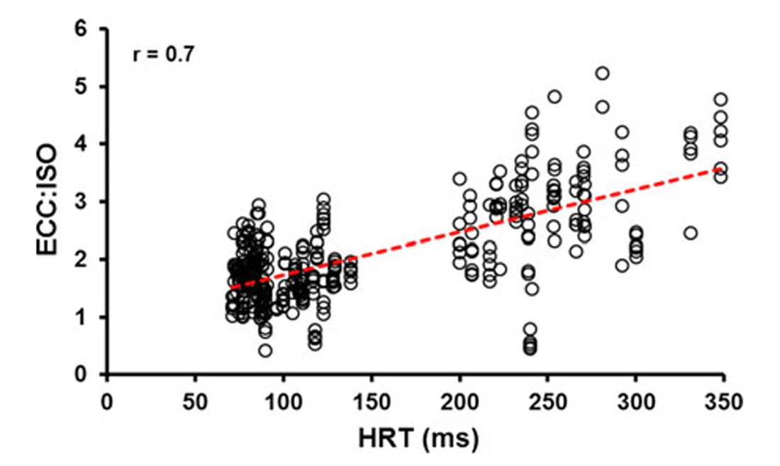 Figure: The relationship between muscle relaxation speed (HRT) and the ratio of eccentric to isometric force. There was a strong relationship between muscle speed and the maintenance of eccentric strength such that individuals with slower muscle properties had a greater eccentric to isometric force ratio. To resist the aging process, there may be some truth in just being stubborn to the natural degeneration of the neuromuscular system. “It's called stubborn-ness. He's more stubborn to push the weights against gravity than gravity is in pulling them down. We should all be so stubborn.” Either way you look at it, aging of the human neuromuscular system is a non-linear process and there are some impressive mechanisms behind the scenes fighting to maintain function and independence into old age. 
0 Comments
By Avery Hinks When performing exercises like a wall-sit, a plank, or holding a box, your muscles are active and producing force, but not creating movement.  In the above exercises, muscles are performing “isometric” contractions, contracting without moving the joints they’re connected to. These exercises are different from exercises that involve movement, such as squats, push-ups, or most exercises you’d see at a gym. In those cases, muscles are instead performing “concentric” and “eccentric” contractions. 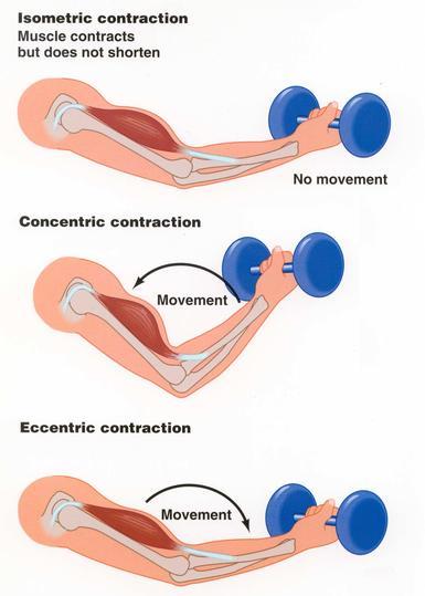 You could argue that exercises involving concentric and eccentric contractions have better applicability to sports and everyday life, and you’d be correct! When you kick a ball, you are performing concentric contractions of your quadriceps. When you walk up the stairs, your legs are performing concentric contractions. When you lift an object off the floor, you’re performing concentric contractions of your arms and legs. When you set the object back down, those same muscles are performing eccentric contractions.  However, what if someone has a limited range of motion, such as while recovering from an injury? In that case, it would be harder to perform exercises involving concentric and eccentric contractions. Here, strength training with isometric exercise is an important alternative. Additionally, some sports do in fact require isometric strength. For example, when using grip strength in mountain climbing, resisting an opponent in wrestling, or stabilizing the body during skiing.  But the benefits of isometric strength training may extend beyond performance in isometric actions. Our lab has shown that isometric training can improve performance during movement as well! Our isometric strength training interventionIn 2019, we conducted an isometric training study with a wide variety of measurements that we published in three separate papers. Seven men and six women participated in 8 weeks of isometric strength training 3 days per week. The muscle group they performed strength training on was the “dorsiflexors,” which are responsible for pulling the top of your foot closer to your shin. The “tibialis anterior” is the primary dorsiflexor muscle, so focusing on the dorsiflexors allowed us to target mainly that one muscle during training. Our setup for this training program is pictured below. 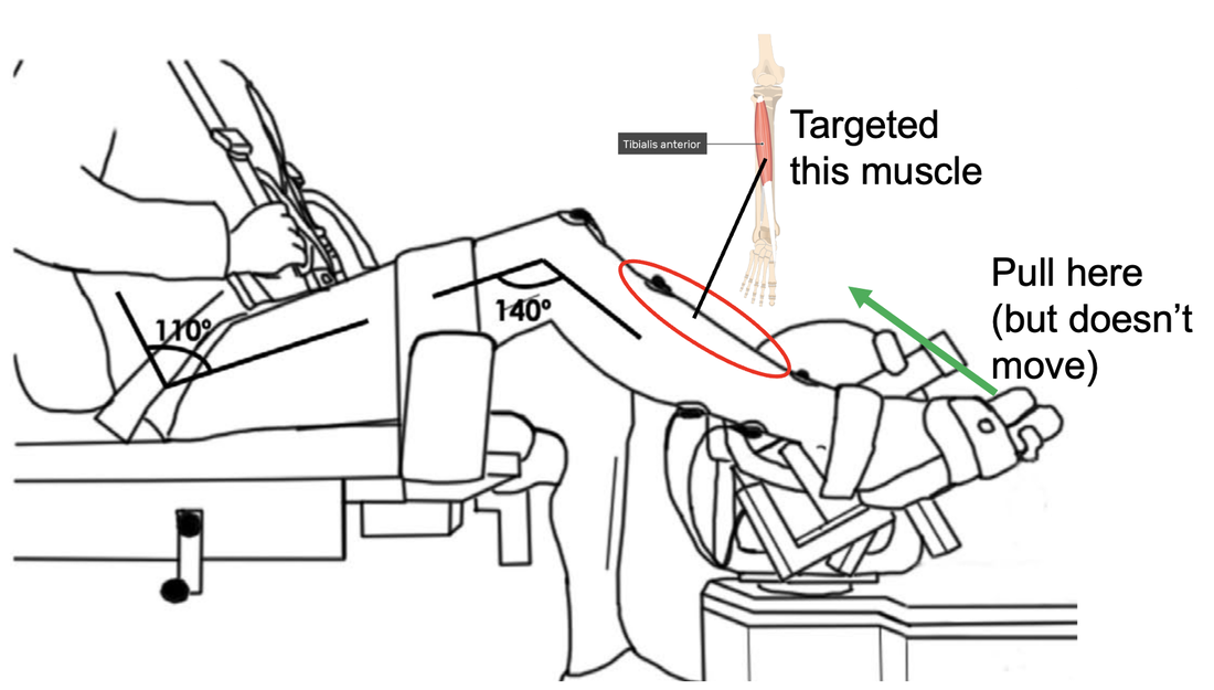 Additionally, we wanted to investigate whether the muscle length used during isometric training can make a difference. To do this, each participant trained one of their legs with the tibialis anterior at a long muscle length, and the other leg with the tibialis anterior at a short muscle length. 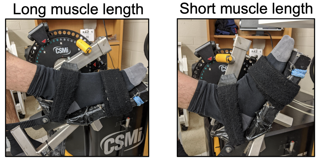 Benefits for muscle structure and isometric strengthMuscle thickness and fascicle pennation angle (PA on the graph below) measured by ultrasound can provide an indication of changes in muscle mass. Following training at both muscle lengths, the thickness and pennation angle of the tibialis anterior increased, as shown below. 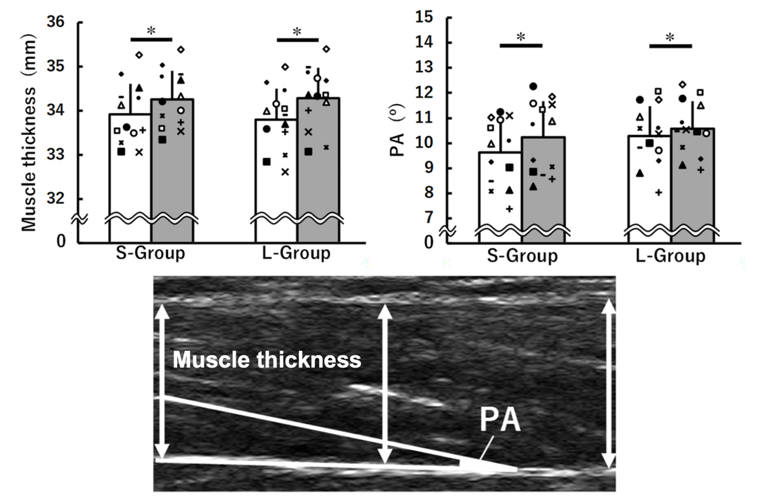 Figure adapted from Akagi et al. (2020), Journal of Applied Physiology. S-Group = training at a short muscle length. L-Group = training at a long muscle length. PA = Pennation angle. White represents before training, while grey represents after training. Muscle thickness and pennation angle also often relate to a muscle’s isometric strength (for more information, see our previous knowledge translation). Correspondingly, maximum isometric strength of the dorsiflexors (“MVC Torque” on the graph below) also increased by about 10% following training at both muscle lengths. These improvements in strength are indicated by the red line on the graph below, which represents the average of all participants. 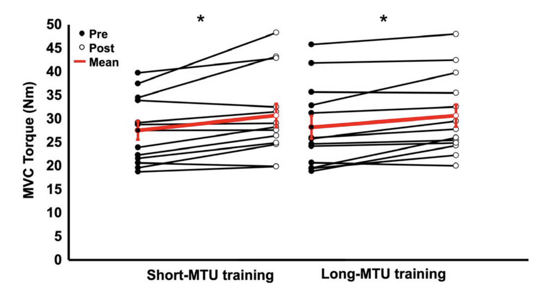 Figure from Hinks et al. (2020), Scandinavian Journal of Medicine and Science in Sports. Short-MTU training = isometric training at a short muscle length; Long-MTU training = isometric training at a long muscle length. The above measurements of isometric strength were obtained at only one joint angle. This distinction is important because, in real life, the body needs to generate isometric strength at more than one joint angle. When we looked into strength adaptations at other joint angles, we observed different results between training at a short muscle length and training at a long muscle length! First, a quick lesson on what we call the “force-length relationship.” For a muscle to generate force, proteins called actin and myosin must bind together. This phenomenon occurs in microscopic units called sarcomeres, which there are thousands of within a whole muscle. 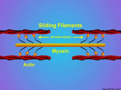 When a muscle is in a stretched or shortened position, these sarcomeres stretch and shorten as well. In stretched or shortened positions, it is harder for actin and myosin to bind together and produce force. With this in mind, force initially increases with increasing muscle length, and we call this the “ascending limb.” There is then a range of muscle lengths in which strength is optimal, called the “plateau region.” Lastly, force decreases as muscle length continues to increase, and we call that the “descending limb.” The width of the plateau region is especially important because it tells us the range of joint angles at which strength is close to optimal. 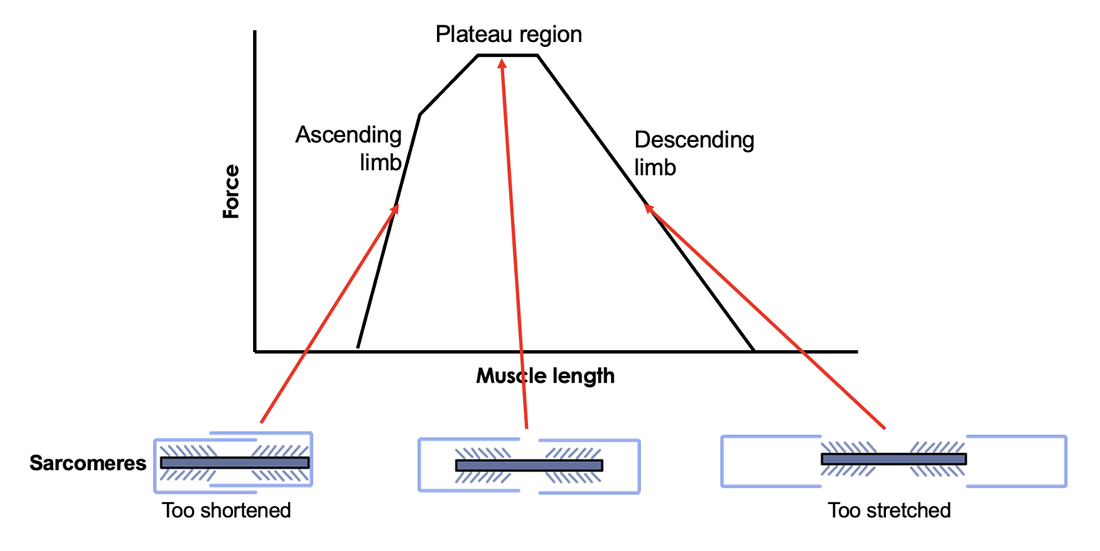 We investigated how the shape of the force-length relationship changed following isometric training at a short compared to a long muscle length. While training at a short muscle length improved strength at some joint angles, the width of the plateau region did not change. Following training at a long muscle length, however, the width of the plateau region widened considerably (indicated by the red box on the graph below). 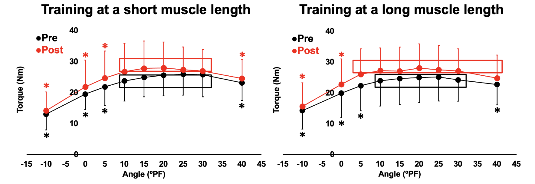 Figure adapted from Akagi et al. (2020), Journal of Applied Physiology. Torque is the measurement of isometric strength. In other words, isometric training at a long muscle length can bring strength close to optimal across a wider range of joint angles. More importantly, it can improve strength at joint angles other than the angle used in training! Widening of the force-length relationship is often associated with in an increase in muscle fascicle length (FL on the graph below). We only observed an increase in fascicle length following isometric training at a long muscle length, so with that in mind, the widening of the plateau region is not surprising. This elongation of muscle fascicles likely occurred because the muscle needed to adapt to acting at a long muscle length during training. 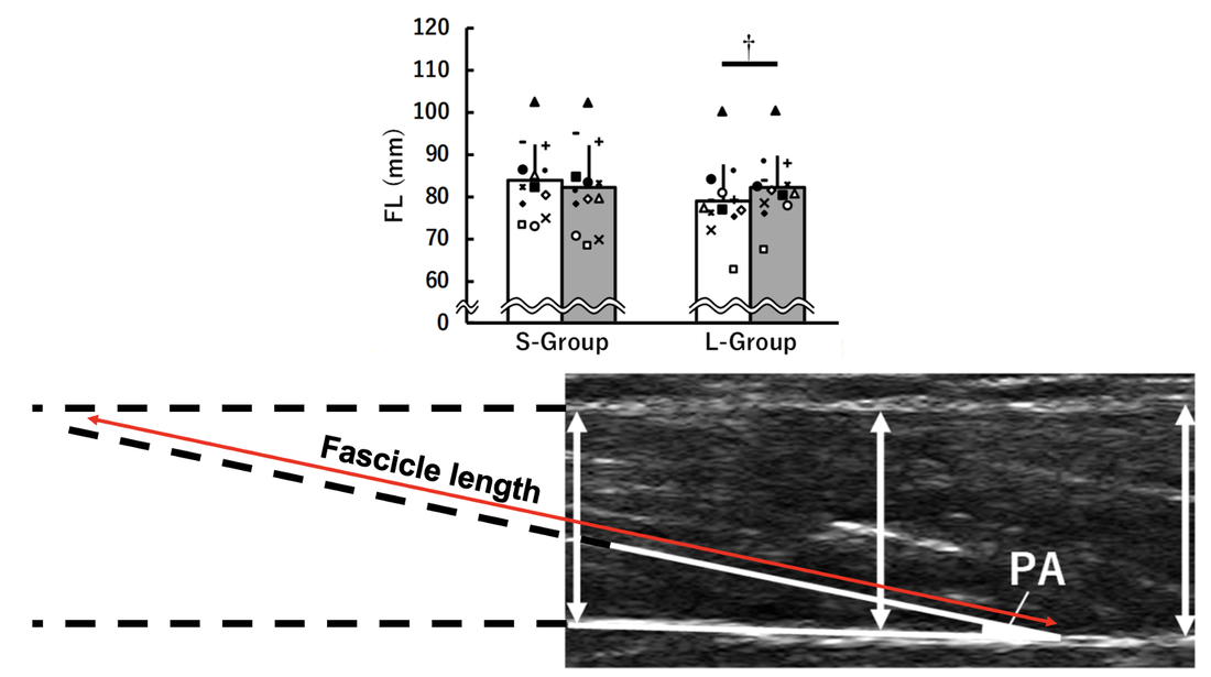 Figure adapted from Akagi et al. (2020), Journal of Applied Physiology. S-Group = training at a short muscle length. L-Group = training at a long muscle length. FL = Fascicle length. White represents before training, while grey represents after training. Does isometric training improve muscle performance during movement? Muscle strength is not only measured in isometric contractions. As mentioned earlier, concentric contractions may be more applicable to everyday movements. We saw that isometric training can also improve strength during concentric contractions (called “dynamic torque” in the graph below). This result did not differ between training at a short and long muscle length. 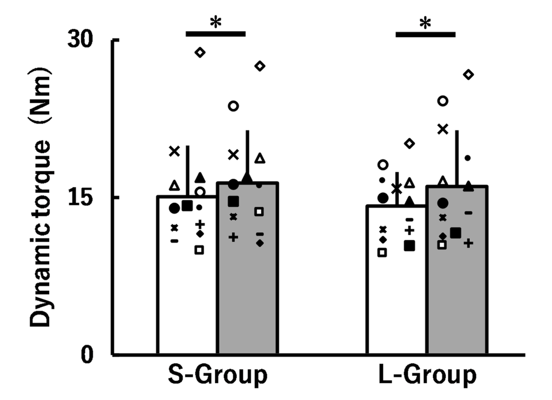 Figure from Akagi et al. (2020), Journal of Applied Physiology. S-Group = training at a short muscle length. L-Group = training at a long muscle length. White is from before training, while grey is from after training. We can also investigate a muscle’s performance during movement by assessing maximum power. Power equals the force produced by the muscle during movement multiplied by the velocity of the movement. Therefore, maximum power incorporates both the strength and the speed of a muscle. This cross between strength and speed is important for explosive movements, such as jumping, sprinting, or powerlifting.  We assessed maximum muscle power in four different conditions of movement:
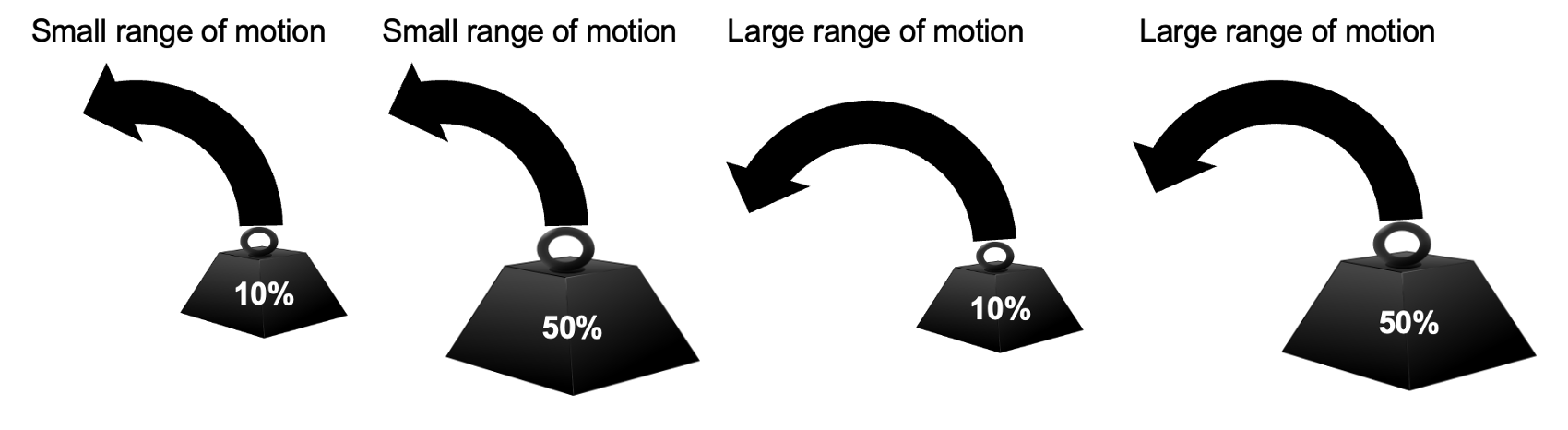 Conditions using a heavier weight and a larger range of motion are intended to be more difficult. Following isometric training at a short muscle length, maximum power only increased in the two small range of motion conditions. Following training at a long muscle length, maximum power increased in the small range of motion conditions even more, and also increased in the large range of motion, 10% weight condition. These results are shown in the graph below, with the red lines representing the average of all participants. 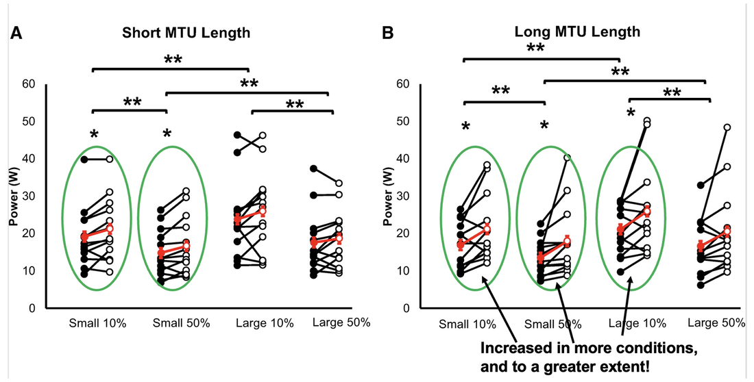 Figure adapted from Davidson et al. (2022), Journal of Applied Physiology. Short MTU length = training at a short muscle length. Long MTU length = training at a long muscle length. We can also assess a muscle’s performance during concentric contractions by looking at the “rate of velocity development.” Rate of velocity development is basically just acceleration (like what you do with your car when merging onto a highway), and describes how fast a muscle can increase its speed. This measurement may seem trivial, but it has applications in everyday life. Most prominently, if you suddenly fall, your muscles must accelerate to catch you.  With both isometric training groups combined, we observed increases in rate of velocity development (RVD in the graph below) during all four concentric contraction conditions. 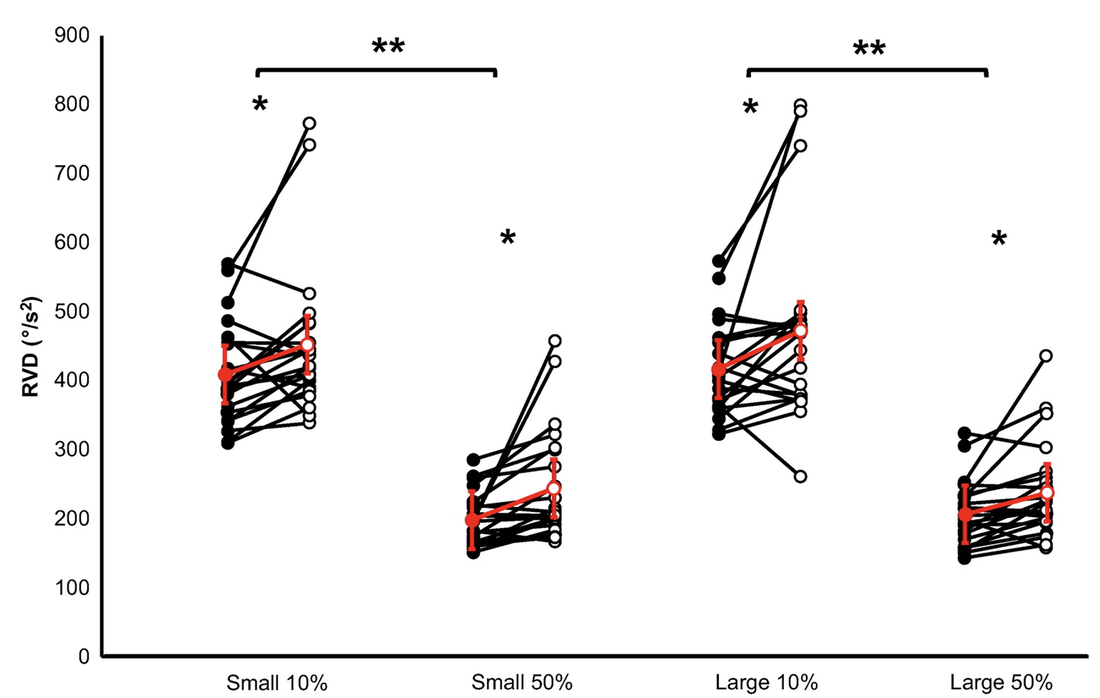 Figure from Davidson et al. (2022), Journal of Applied Physiology. Altogether, even though isometric training involves only static contractions, it can improve performance in dynamic contractions—especially when training is performed at a long muscle length! Conclusion Isometric strength training has sport-specific applications and may be useful during recovery from an injury that restricts range of motion. Some people may also prefer the static nature of isometric training compared to conventional resistance training (see the photo below from isophit.com). And that’s okay! Our study determined that isometric training is a viable option for eliciting positive adaptations in muscle structure and improving performance in both static and dynamic actions. When isometric training is performed at a long muscle length, these adaptations seem to be even more pronounced!  People performing an isometric training workout. From isophit.com. References Akagi R, Hinks A, Power GA. Differential changes in muscle architecture and neuromuscular fatigability induced by isometric resistance training at short and long muscle-tendon unit lengths. J Appl Physiol (1985). 2020 Jul 1;129(1):173-184. doi: 10.1152/japplphysiol.00280.2020. Epub 2020 Jun 18. PMID: 32552430; PMCID: PMC7469237.
Davidson B, Hinks A, Dalton BH, Akagi R, Power GA. Power attenuation from restricting range of motion is minimized in subjects with fast RTD and following isometric training. J Appl Physiol (1985). 2022 Feb 1;132(2):497-510. doi: 10.1152/japplphysiol.00688.2021. Epub 2022 Jan 13. PMID: 35023762. Hinks A, Davidson B, Akagi R, Power GA. Influence of isometric training at short and long muscle-tendon unit lengths on the history dependence of force. Scand J Med Sci Sports. 2021 Feb;31(2):325-338. doi: 10.1111/sms.13842. Epub 2020 Oct 19. PMID: 33038040. By Avery Hinks Starting around age 60, noticeable changes in muscle function often manifest. It’s January here in Guelph, Ontario, so I’ll use a winter example. You awake after a night of snowfall and need to clear your driveway. As you do so, you might notice it’s harder to shovel snow. The salt bags you use to spread salt might also feel heavier than they used to. When you’re done, on your way back up your front step, you might slip on a patch of ice, and notice your limbs move slower to catch your fall.  These impairments in muscle function stem from the fundamental biomechanics of your muscles. Specifically, the abilities to produce force, velocity, and power. Several changes associated with aging contribute to these impairments. Namely, there are changes in the connection between the brain and the muscles, the biochemical processes occurring in the muscles, and the muscles' structure.  To make this knowledge translation a digestible length, I will focus only on how changes in muscle structure contribute to deficient muscle function in old age. The other contributors will I’m sure be covered in a future knowledge translation! What does a muscle look like, structurally?Whether you are younger or older, the structure of any of your muscles can be viewed as a hierarchy. Think of a muscle’s structure as an inverted pyramid.  At the top, there is the muscle as a whole. Looking closer, many smaller structures called muscle fascicles comprise that whole muscle. I say “smaller,” but muscle fascicles are easily visible without a microscope. The next time you cook chicken for dinner, pay close attention as you slice it. You will be able to see distinct lines running through the meat. Those are fascicles! There are mainly two properties we measure regarding muscle fascicles. In the image below, you can see that the fascicles are at an angle to the borders of the muscle. We call this the “pennation angle.” We also measure the “fascicle length,” which is exactly how it sounds: the length of a fascicle from end to end. At this level of muscle, we can also characterize structure with "muscle thickness," which provides an indication of muscle size. In humans, these measurements are usually captured using ultrasound, as shown below. 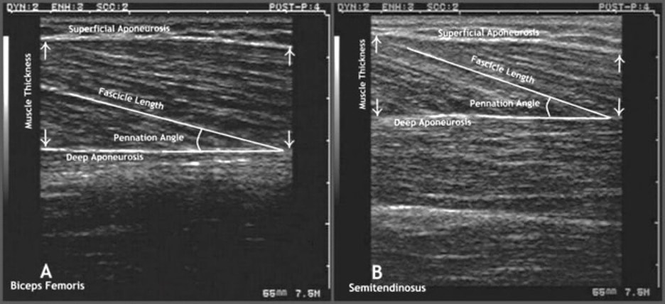 Figure from Oliveira et al. (2016), Research on Biomedical Engineering. To appreciate the relationship between muscle fascicle length, pennation angle, and thickness, we can think in terms of geometry. For a fascicle to be longer, there must be a smaller pennation angle, or the thickness of the whole muscle must increase, keeping pennation angle the same. 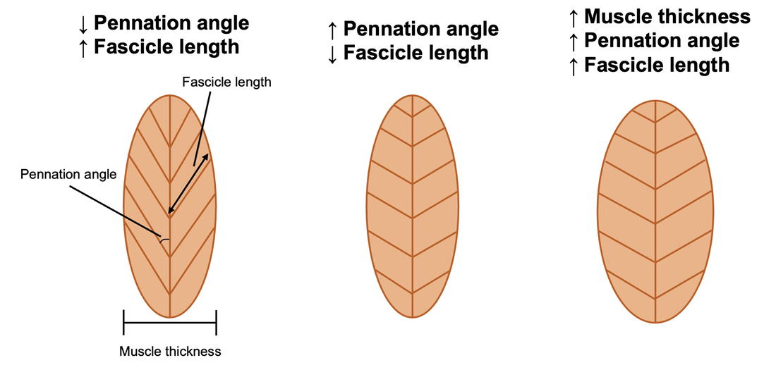 Going further down the pyramid, a muscle fascicle is comprised of many muscle fibres. A muscle fibre is comprised of the tiny structures that allow a muscle to produce force. These structures are called sarcomeres.  When you activate your muscle for a required task, proteins in the sarcomere called myosin and actin bind together. These proteins then pull the outer edges of the sarcomere closer together to generate force. Right now, look at your bicep muscle and flex it. Do you see how it becomes shorter and more tense? That is the result of thousands of sarcomeres in your bicep contracting altogether. 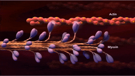 We can look at the arrangement of sarcomeres in a muscle fibre in two ways. First, they are arranged along the fibre’s length, in the direction that sarcomeres pull when producing force. The number of sarcomeres from end to end along a muscle fibre is called the “serial sarcomere number”. Second, sarcomeres are arranged side to side, parallel to each other in the muscle fibre. We call this (unsurprisingly) the “parallel sarcomere number.” A greater serial sarcomere number means a muscle fibre is longer, while a greater parallel sarcomere number means a muscle fibre is wider. 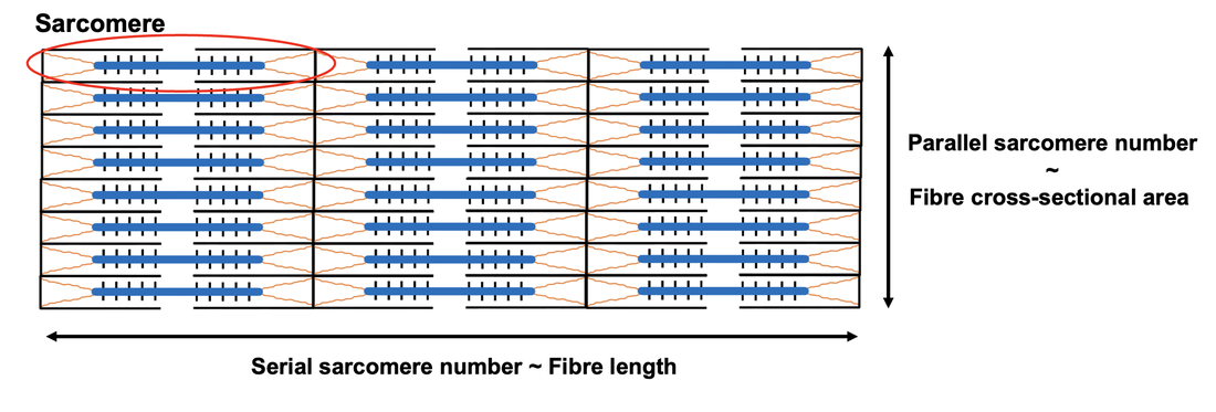 Considering the pyramid of muscle structure, we can appreciate that serial and parallel sarcomere number can influence the appearance of muscle structure at a larger scale. Serial sarcomere number contributes to a muscle’s fascicle length, while parallel sarcomere number contributes more to a muscle’s pennation angle and thickness. What does muscle structure mean for muscle function? There are arguably three main measures to consider when discussing fundamental muscle function. First, there is strength, which is measured as maximum force production. Second, there is speed, which is measured as a muscle's maximum shortening velocity. Lastly, there is power output, which combines strength and speed together. Each of these measures is influenced by muscle structure. Picture yourself trying to pull a giant rock with a rope. Seems hard, right? Well, what if other people join in, each pulling from their own rope, parallel to yours? It will become easier because your pull altogether is stronger than one person alone. 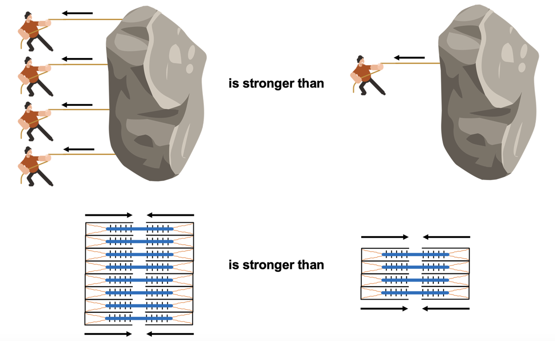 When sarcomeres contract so your muscle can lift an object, it works the same! With more sarcomeres in parallel (and on a larger scale, greater pennation angle), your muscle can produce more force. Opposite to parallel sarcomere number, serial sarcomere number instead contributes to maximum velocity. This relationship is best demonstrated with math. I’ll walk you through it. While a muscle typically has thousands of sarcomeres in series, below are two hypothetical muscles: one with three sarcomeres, and one with six. As well, sarcomeres are very small (about 2 thousandths of a millimetre), but for the sake of making the math easy, let’s say each sarcomere is 1 millimetre long. 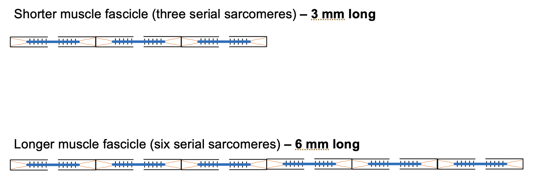 Now let’s say each sarcomere shortens to half its original length, as shown below. Velocity is measured in units of distance over time, so we’ll also say this shortening occurs in 1 second. 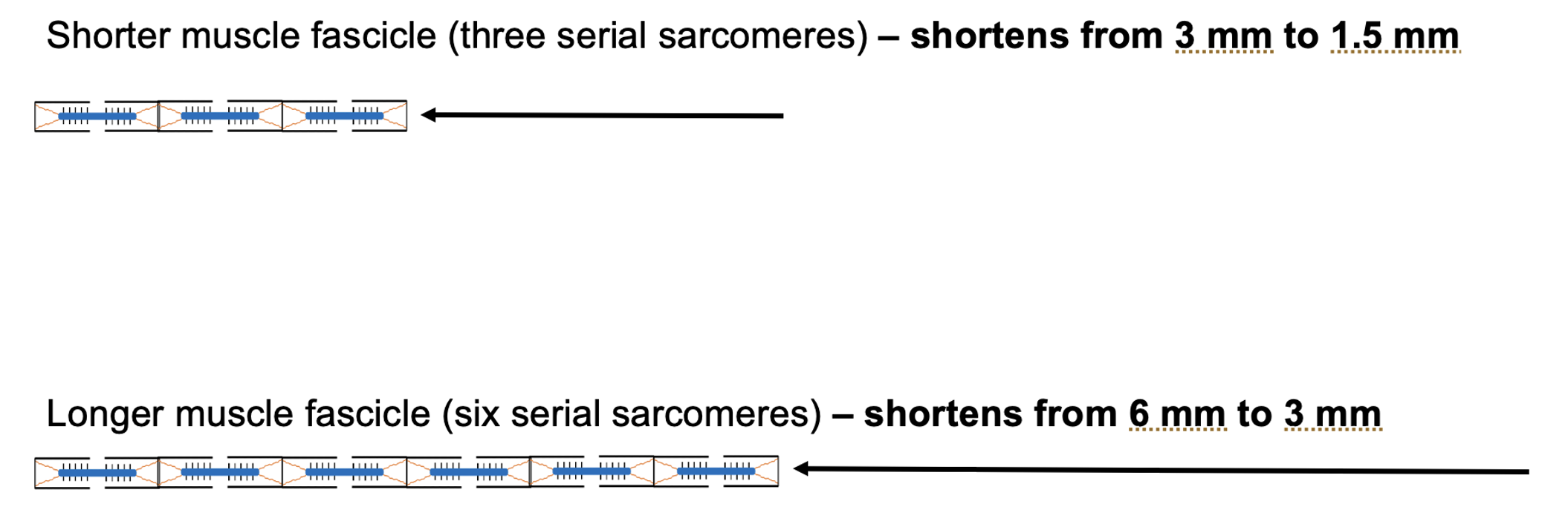 The shorter fascicle (top) shortened from 3 mm to 1.5 mm in 1 second, giving it a velocity of 1.5 mm/s. The longer fascicle (bottom) shortened from 6 mm to 3 mm, giving it a faster velocity of 3 mm/s. This example shows that for the same amount of shortening in each sarcomere, a muscle with more serial sarcomeres can shorten faster! Lastly, there is maximum muscle power output. Simply put, power is equal to force times velocity. Therefore, muscle power is important in tasks involving both strength and speed. For example, when jumping as high as you can.  Remember, parallel sarcomere number contributes to maximum force production, and serial sarcomere number contributes to maximum shortening velocity. Therefore, both these aspects of muscle structure are important in maximum muscle power. How does muscle structure change with age?A study by Narici and colleagues in 2003 was one of the first to show how muscle structure changes in old age. They showed that 70 to 81 year old men had 10% shorter fascicles and 13% smaller pennation angles in a muscle of the lower leg (the calf) than 27 to 42 year old men. Since then, several other studies have observed similar results in other muscles, and also in women. 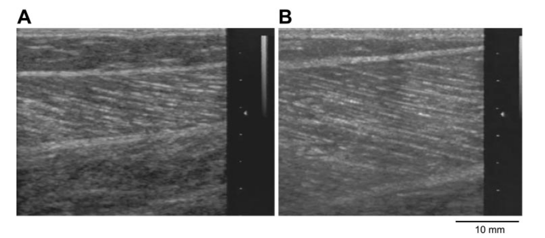 "A" shows an ultrasound image of the muscle structure of an older man, while "B" shows that of a younger man. Figure from Narici et al. (2003), Journal of Applied Physiology. Given these changes in muscle structure, the functional changes observed in old age are not surprising. A study by Hughes and colleagues in 2001 assessed strength of the knee extensor (kicking) muscles in 120 individuals ranging from 46 to 78 years old. They showed the strength of these muscles declines 14% per decade of life on average. Similar declines have also been observed for maximum shortening velocity and power output. The figure below shows muscle shortening velocity and power when lifting a range of weights (“Load” on the graphs) in young, old, and very old men. This figure demonstrates clear reductions in both muscle speed and power throughout the lifespan. 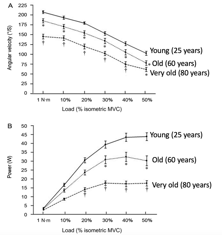 Figure from McNeil et al. (2007), Journal of Applied Physiology. Similar results for muscle speed and power were also shown in women in a study by Macaluso and colleagues. Older women had a 21% slower maximum velocity and generated 61% less power in their legs than younger women. 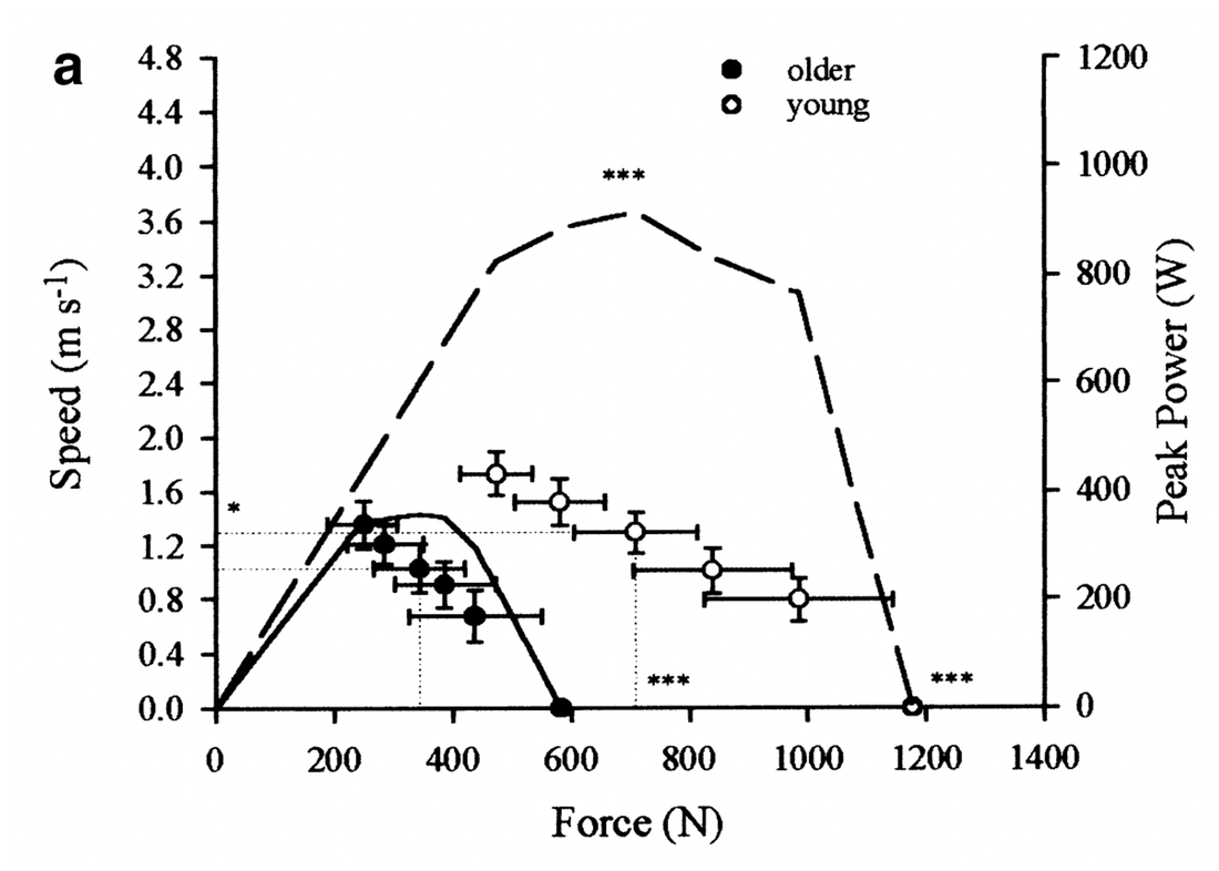 Solid line = peak power of older women. Dashed line = peak power of young women. Black dots = speed of older women. White dots = speed of young women. Figure from Macaluso et al. (2003), European Journal of Applied Physiology. Is there any hope?Of course!  Returning to the study that investigated 120 subjects by Hughes and colleagues, one of their figures sticks out.  Figure from Hughes et al. (2001), Journal of Gerontology. The figure above shows strength reductions in the men and women investigated in Hughes’ study in four different muscle groups. The percentage values represent the proportion of individuals who did not exhibit declines in strength over time. This likely depends on lifestyle. In other words, the old saying, “Use it or lose it,” holds merit. To that end, many studies have depicted figures like the one below, showing how exercise can delay the reduction in muscle strength (and with it, the onset of frailty) with aging.  Figure from Booth and Zwetsloot (2009), Scandinavian Journal of Medicine and Science in Sports. It is clear that training earlier in life can delay the decline in muscle strength. With that said, positive adaptations in muscle structure and function are still possible in old age. For example, a study by Reeves and colleagues in 2004 submitted older men and women (on average 74 years old) to resistance training of the legs 3 days per week for 14 weeks. This training program resulted in a 10% increase in maximum leg strength. Correspondingly, this training program induced a 10% increase in fascicle length and a 30% increase in pennation angle in one of the leg muscles.  Conclusion As we age, our muscles experience decreases in fascicle length and pennation angle. These changes in muscle structure likely contribute to the impairments in muscle strength, velocity, and power output seen in old age. Resistance training earlier in life can delay these changes in muscle structure and function—but perhaps more importantly, resistance training during old age can also reverse these changes to an extent. Our lab is currently looking into the distinct links between changes in muscle structure and changes in muscle function—and their adaptability with training—in old age.
If you are on the older side, and find yourself feeling weak shovelling your driveway after a snowstorm, I hope you have learned that you still have the capacity to grow stronger! References Booth, F. W., & Zwetsloot, K. A. (2010). Basic concepts about genes, inactivity and aging. Scandinavian journal of medicine & science in sports, 20(1), 1-4. Hughes, V. A., Frontera, W. R., Wood, M., Evans, W. J., Dallal, G. E., Roubenoff, R., & Singh, M. A. F. (2001). Longitudinal muscle strength changes in older adults: influence of muscle mass, physical activity, and health. The Journals of Gerontology Series A: Biological Sciences and Medical Sciences, 56(5), B209-B217. Macaluso, A., & De Vito, G. (2003). Comparison between young and older women in explosive power output and its determinants during a single leg-press action after optimisation of load. European journal of applied physiology, 90(5), 458-463. McNeil, C. J., Vandervoort, A. A., & Rice, C. L. (2007). Peripheral impairments cause a progressive age-related loss of strength and velocity-dependent power in the dorsiflexors. Journal of applied physiology, 102(5), 1962-1968. Narici, M. V., Maganaris, C. N., Reeves, N. D., & Capodaglio, P. (2003). Effect of aging on human muscle architecture. Journal of applied physiology, 95(6), 2229-2234. Oliveira, V. B. D., Carneiro, S. P., & Oliveira, L. F. D. (2016). Reliability of biceps femoris and semitendinosus muscle architecture measurements obtained with ultrasonography. Research on Biomedical Engineering, 32, 365-371. Reeves, N. D., Narici, M. V., & Maganaris, C. N. (2004). In vivo human muscle structure and function: adaptations to resistance training in old age. Experimental physiology, 89(6), 675-689. By Avery Hinks Often in the field of biomechanics and muscle physiology, we construct graphs of the relationship between one muscle variable and another. For example: the relationship between muscle length and muscle force (the active force-length relationship), the relationship between force and the concentration of calcium in a muscle fibre (the force-pCA relationship), or the relationship between muscle force and contraction speed (the force-velocity relationship). 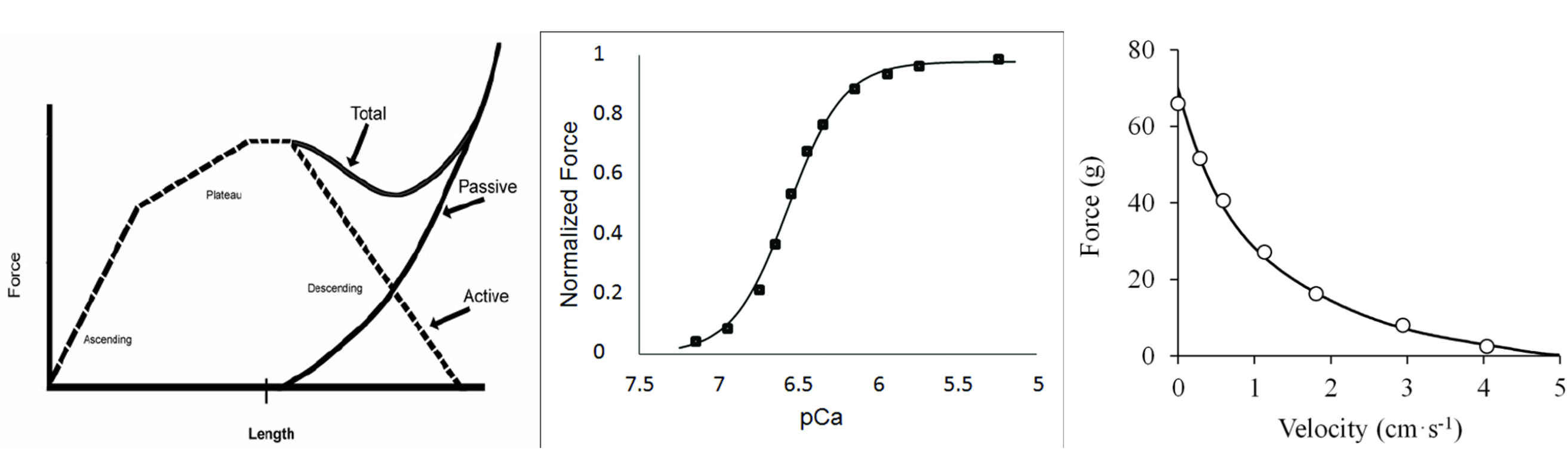 Graphs from: Knudson (2006), Journal of Exercise Science and Physiotherapy; Zhang et al. (2018), Frontiers in Physiology; Alcazar et al. (2019), Frontiers of Physiology. After constructing these relationships from collected data, the question often arises of how to display these data across multiple participants, and make comparisons between groups. For example, a group that completed a training program versus a group that didn’t, or a group of younger versus older individuals. Graphing each collected data point can make statistical analyses difficult. To get around this, many often fit the data to an equation. Fitting data to an equation allows the generation of infinite theoretical data points based on the trends within your data, and the comparison of constants between participants and groups. A prominent example, and the example I will be using throughout this knowledge translation, is the force-velocity relationship. The force-velocity relationship is often fitted to the following equation developed by Hill (1938): 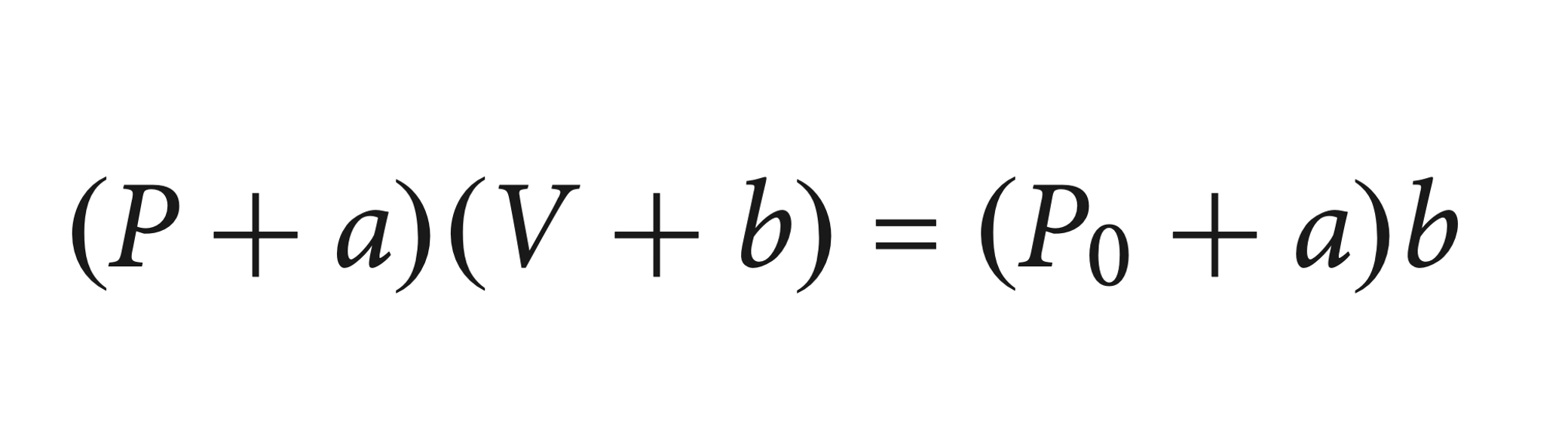 In the equation above, P represents force and V represents velocity. a and b are adjustable constants, with a representing the heat produced during shortening and b representing the increase in energy as force decreases. The first time someone suggested I fit my data to an equation, I was horrified. I’d heard too many stories of people spending hours in coding software such as R or Python. But have no fear! Fitting data to an equation can be easier than it’s made out to be, and you can do it accurately in Excel. Today, I’m going to show you how that works. First, let’s talk about the Force-Velocity RelationshipTo generate strength in muscle, many small proteins called actin and myosin bind to form “cross-bridges”. The formation of these cross-bridges produces force, and that’s what gives our muscle the strength to push, pull, walk, and run.  When lifting an object, muscle undergoes a “concentric” contraction, which means it shortens while producing force. 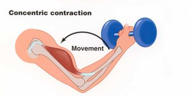 When a muscle shortens very slow, actin and myosin can easily bind each other, leading to near-maximal force production. However, as the muscle shortens faster, more of these actin and myosin filaments slide past each other without the opportunity to bind. Therefore, the ability for muscle to produce force decreases with increasing shortening velocity. From this principle, the force-velocity relationship looks like this: 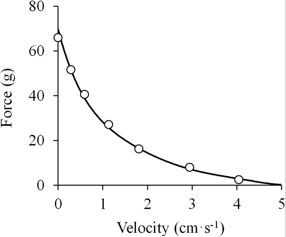 From Alcazar et al. (2019), Frontiers of Physiology. In the graph above, the white circles represent the collected data points, and the line represents the curve generated from fitting the points to Hill’s equation. I have my data points. Now what do I do?After collecting data for muscle shortening velocity across various levels of force, you’re ready to fit them to an equation! I will go through the Excel method step by step. First, make sure you have the “Solver” add-on in Excel turned on. To do this, first click on the “Data” tab.  In the Data tab, all the way to the right, click “Analysis Tools”.  An “Add-ins” pop-up will appear. Check “Solver Add-In” then click “OK”.  You should now see the “Solver” tool in your Data tab.  Now you can get started! The data I’ll be using as an example is from one of the first force-velocity papers, by A.V. Hill in 1938. 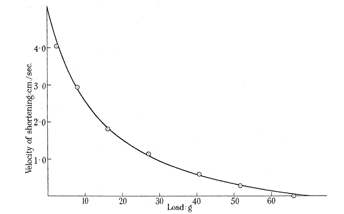 First, you’ll want to make the following column labels: 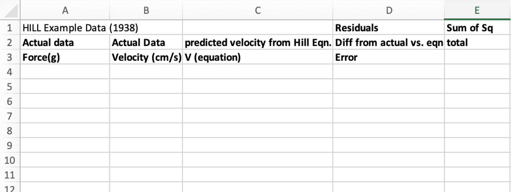 Next, fill in the first two columns with the Force and Velocity data you collected. Additionally, add a box showing the mean (average) velocity value, which will be important later. 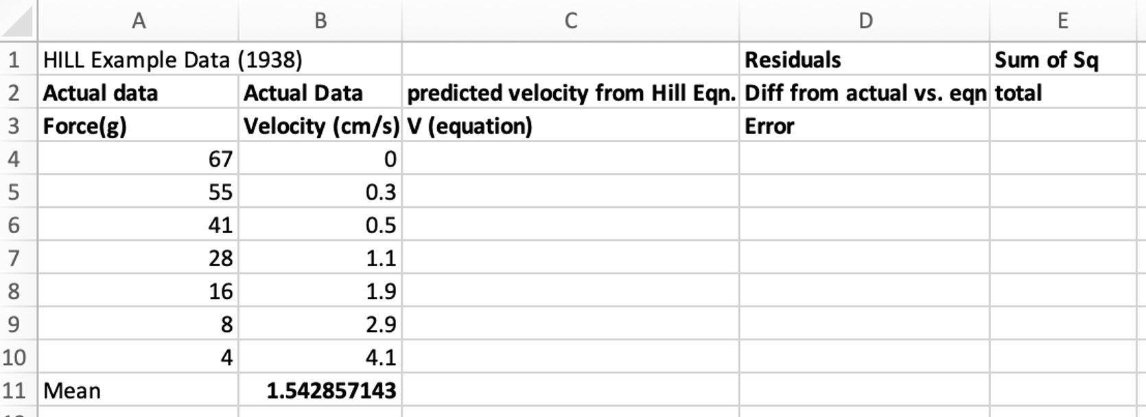 Now we look to Hill (1938)’s equation: We want to use this equation to calculate velocities from given force values. Therefore, before we do anything else, we need to re-arrange this equation to isolate V. If you’ve blocked out everything you learned in 12th grade algebra, do not worry. Here are the steps: (P + a) (V + b) = (Po + a) b If we divide both sides by (P + a), we have: V + b = ((Po + a) b) / (P + a) Now we just have to subtract b from both sides: V = (((Po + a) b) / (P + a)) – b This is the equation we’ll be using for our curve fitting! As a reminder: in this equation, V is the calculated velocity, P is a given force value, Po is the maximum force (i.e., force at 0 velocity), and a and b are adjustable constants. What we want to do with our solver is adjust a and b so that the calculated velocities fit our collected data as best as possible. To do this, we first need to add cells for a, b, and Po. 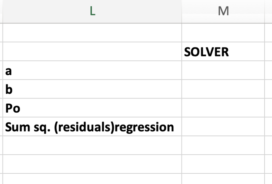 The “Sum sq” cell will come in handy in a moment, too. I recommend placing these cells at about this distance (see below) from the columns we made earlier. You’ll see why over the next few steps. 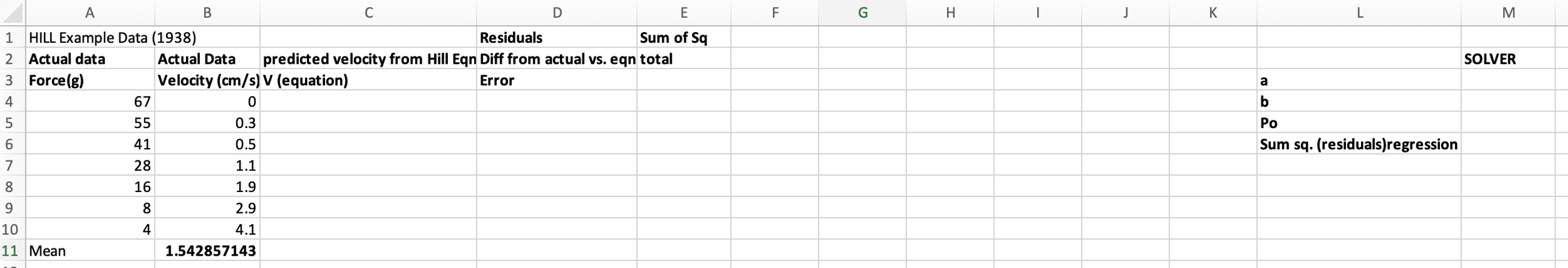 We can now fill the equation in the “Predicted Velocity” column as follows: 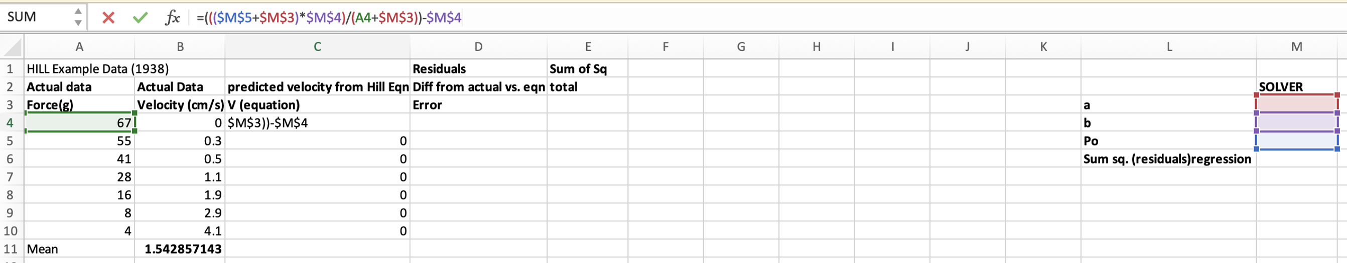 For now, because the constants are empty, all the values come up as 0. To best visualize the curve-fitting in action, we can construct a graph showing two separate plots: one with the collected velocity on the Y-axis and collected force on the X-axis; and one with the calculated velocity on the Y-axis and collected force on the X-axis. Since our predicted velocity column is not filled in yet, it will start out looking like this: 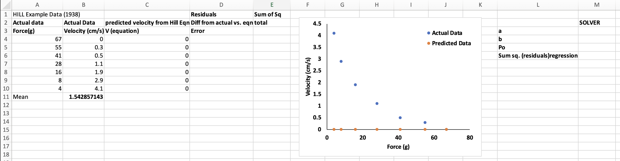 Now we’ll fill in the two remaining columns: “Error” and “Sum of Squares total”. In the Error column, we want the difference between the predicted and collected velocities, so we use the following equation: 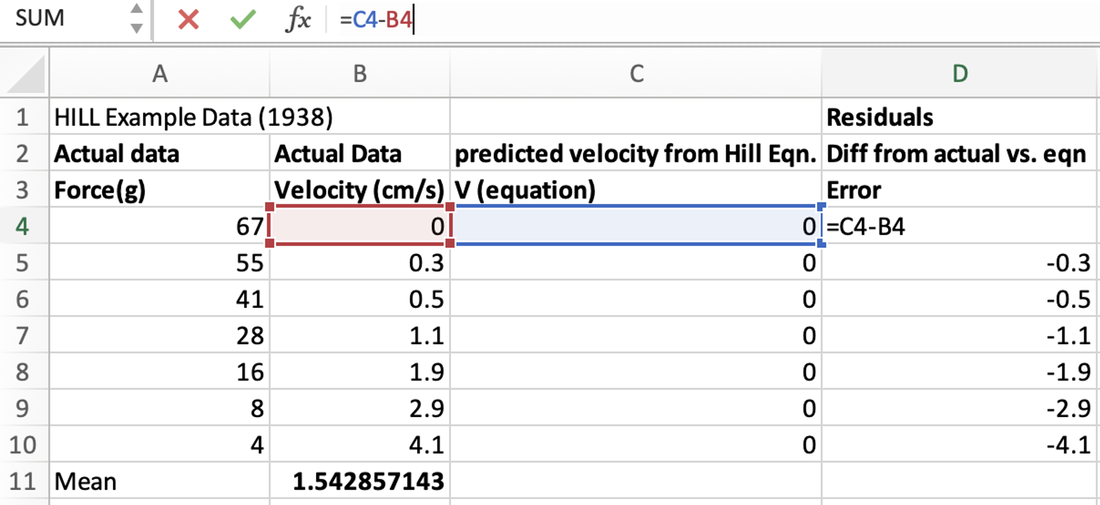 In the Sum of Squares Total column, we want the difference between each collected velocity data point and the mean collected velocity, so we use this equation: 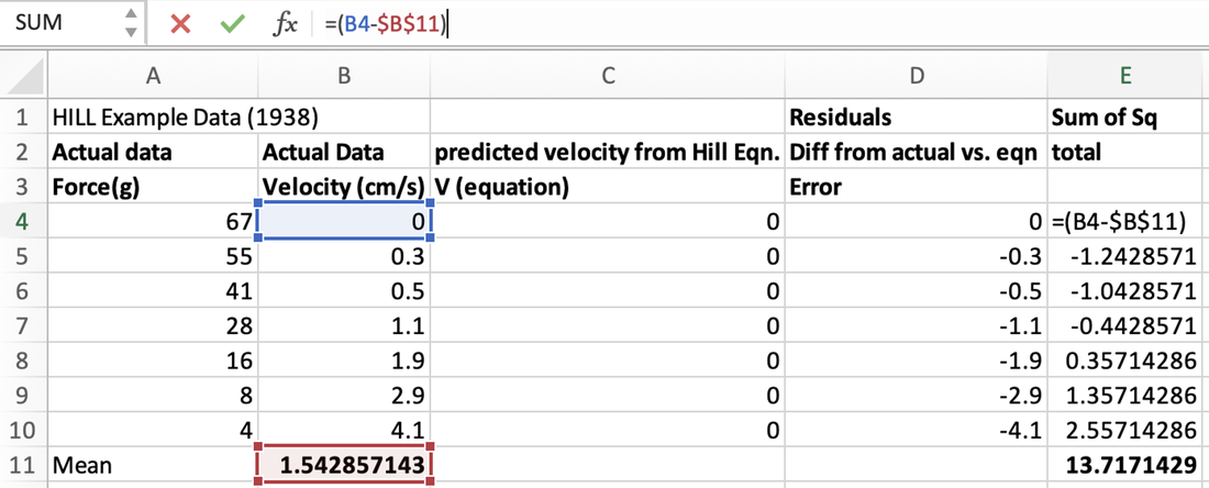 The bolded value below the Sum of Squares Total column is the Sum of Squares Total value. We compute this with the following equation: 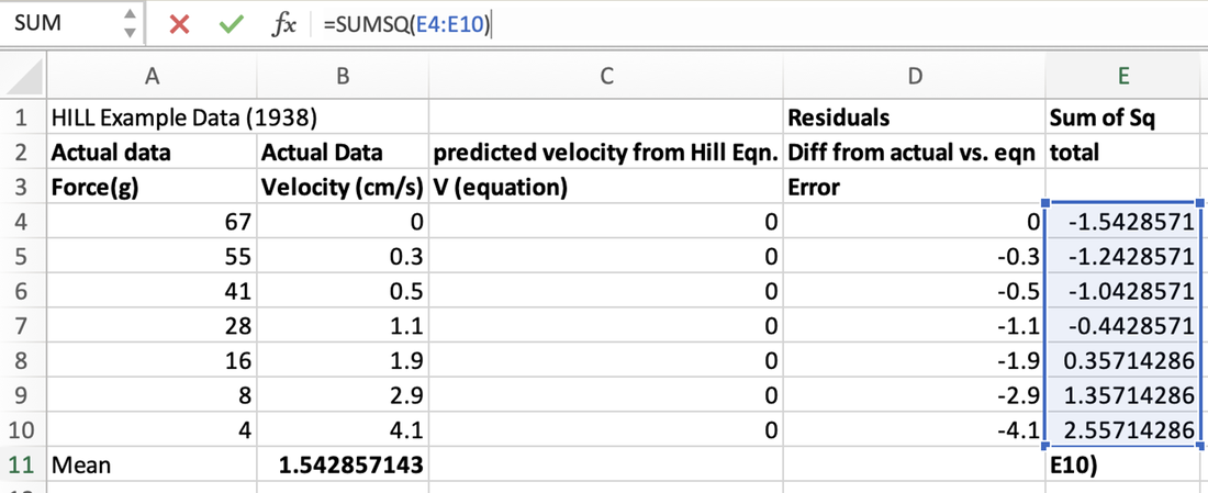 Now that our equations are all setup, we can fill in the constants. For Po, we can see that the maximum force is 67, so that’s what we put there. For a and b, the starting values are mostly arbitrary, but they have to be relatively close to the proper values. What do I mean by this? Basically, you can adjust a and b while watching the orange points on the graph until the trends made by both the orange and blue points are clearly visible. For example, here I’ve started a at 9 and b at 2: 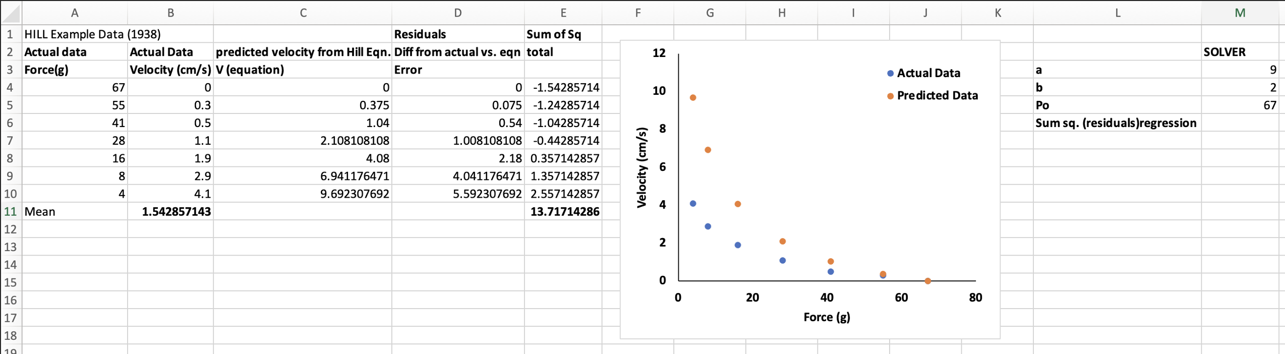 These should be close enough for the Solver to work with. One more step before I employ the Solver. We need to fill in the “Sum of squares residuals” box under Po. This value represents the Sum of Squares of the “Error” column and may be the most important value for the Solver. To compute this, we use the following equation: 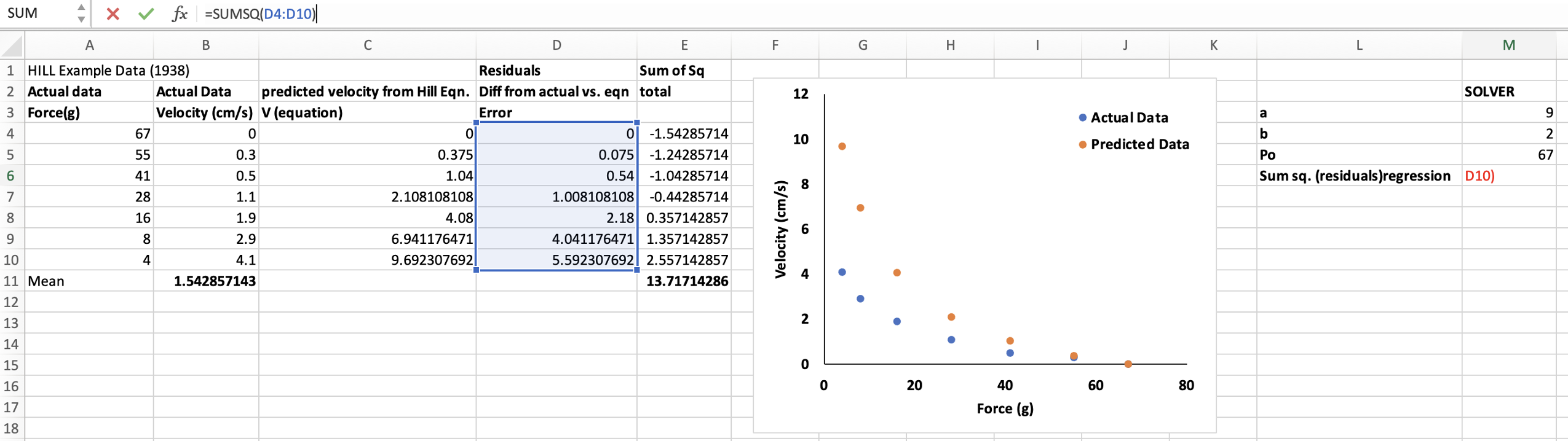 And we end up with a starting Sum of Squares Error of 53.67. This is a very high error value, and makes sense since the orange data points are currently far away from the blue data points. The Solver will work to minimize this Sum of Squares Error to make the predicted values as close as possible to the collected values. 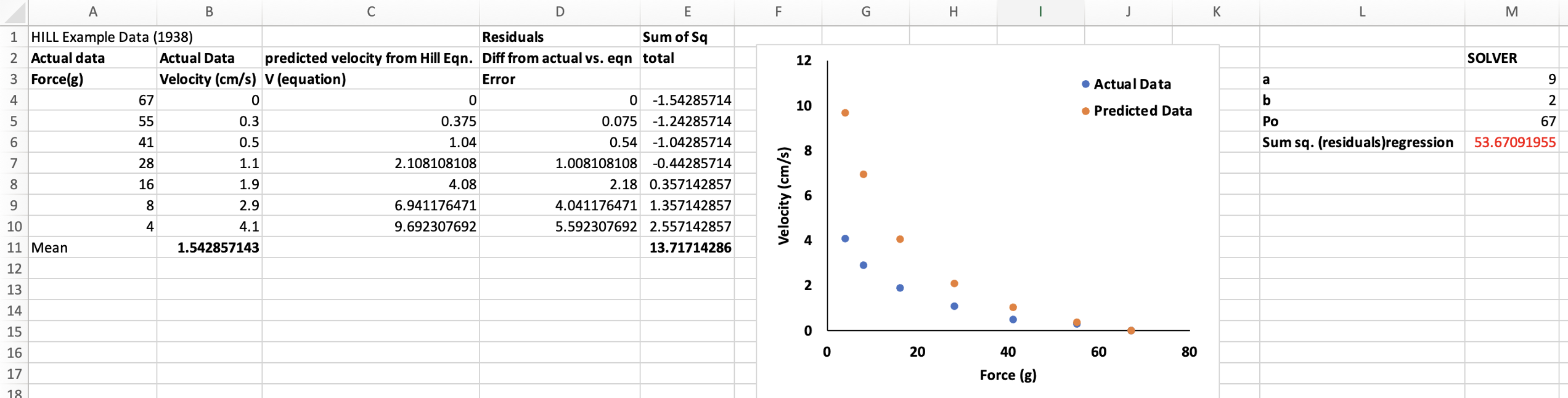 Now, go to the “Data” tab, and open the “Solver”. This window will pop up: 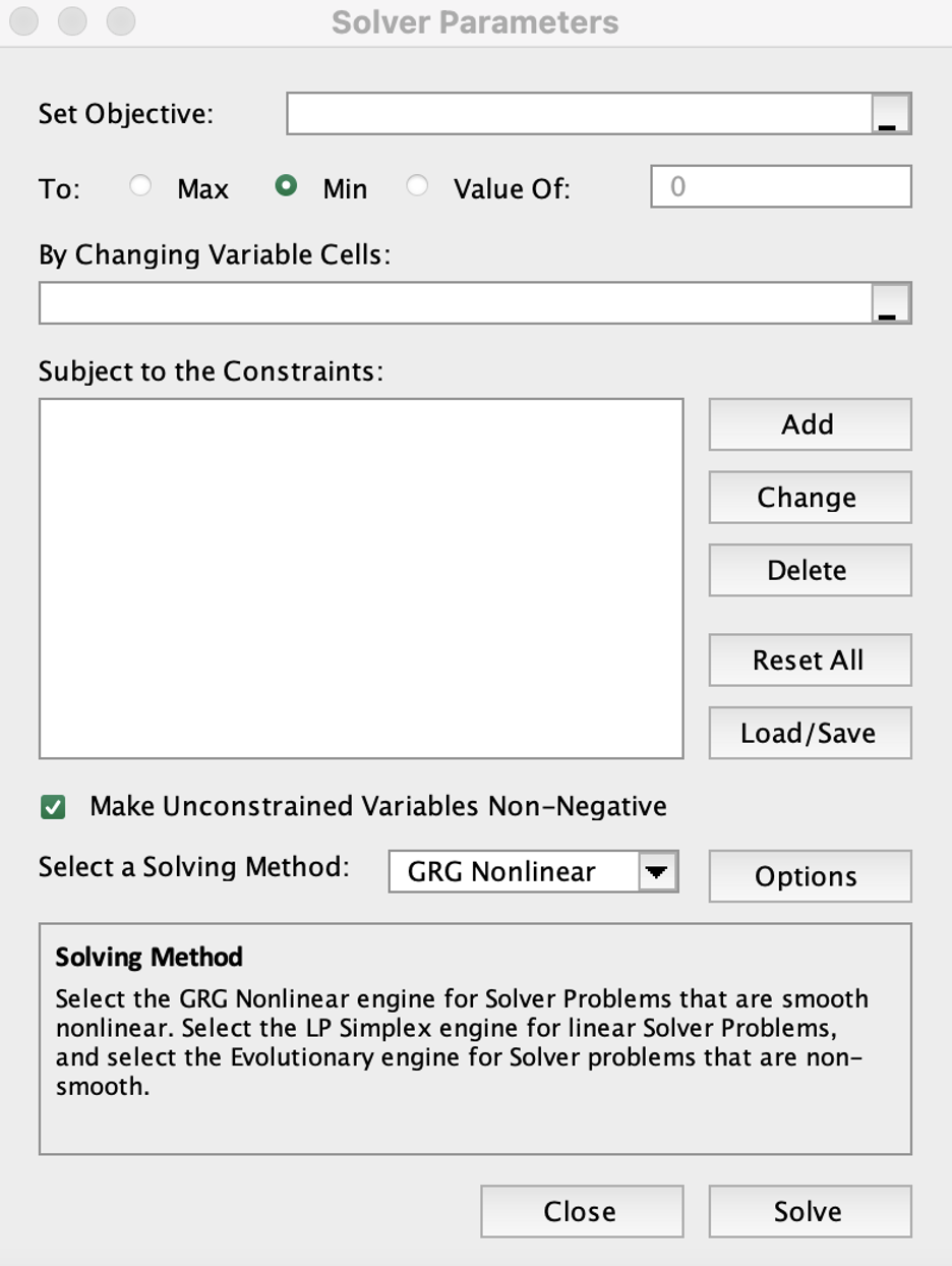 First, we want to set our objective. This will be the Sum of Squares Error cell. We also select “Min” because we want the Solver to minimize this error. 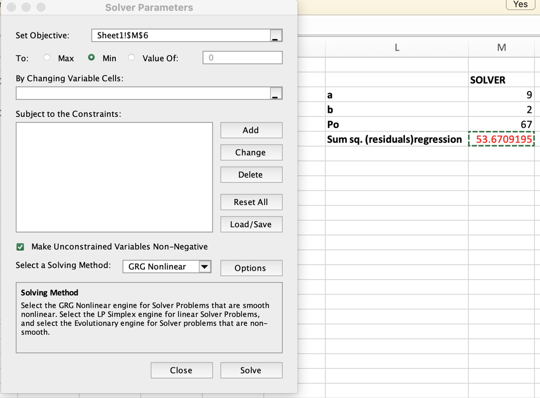 Under “By Changing Variable Cells”, we select the a and b constants, because we want the Solver to adjust these constants to minimize the error. 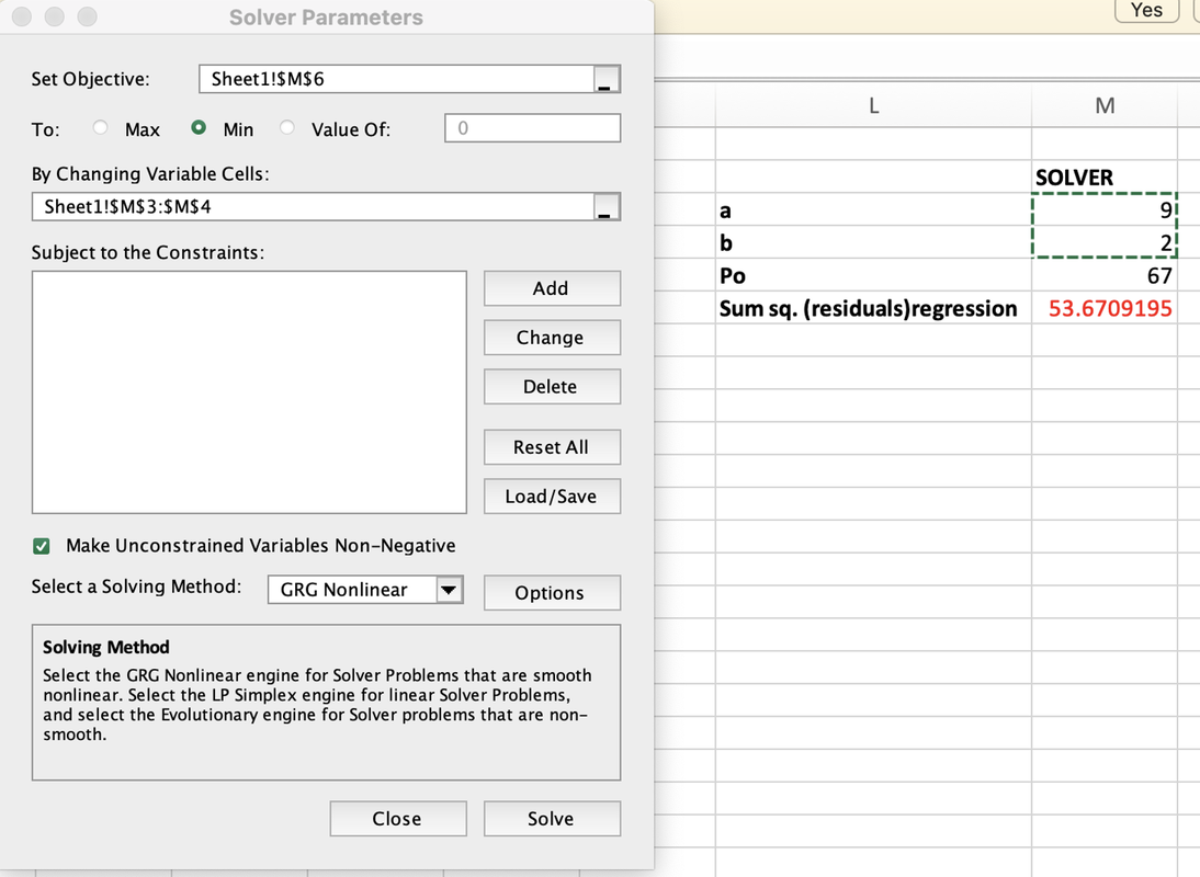 Now we click “Solve”! I’ve recorded a video so you can watch what the Solver looks like in real time: https://drive.google.com/file/d/1lbQQu3ttDt8et-kY8LFrV88GrydB1IIC/view?usp=sharing As you can see, once the Solver is done, a and b have been determined, the Sum of Squares Error has been minimized (from 53.67 to 0.04), and the orange dots fit the blue dots much better! 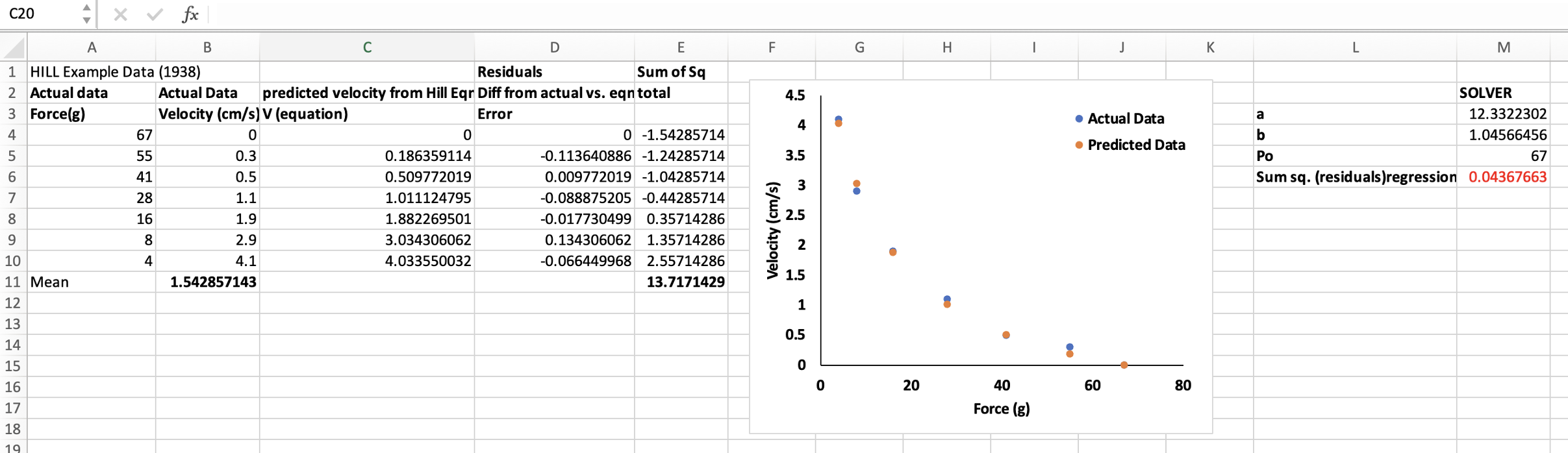 You probably noticed in the video that there are a few things I haven’t added in yet. The first is the R^2 value. This value will tell you how good of a fit your Solved data points are to your collected data points. The maximum R^2 value is 1.0 (meaning a 100% fit), and generally we want at least 0.98 as indication of a good fit. To calculate R^2, we will divide the Sum of Squares Residuals by the Sum of Squares Total, then subtract the result from 1. In Excel, we use this equation:  For this example, we end up with an R^2 of over 0.99, indicating our Solved force-velocity curve fits our data very well! 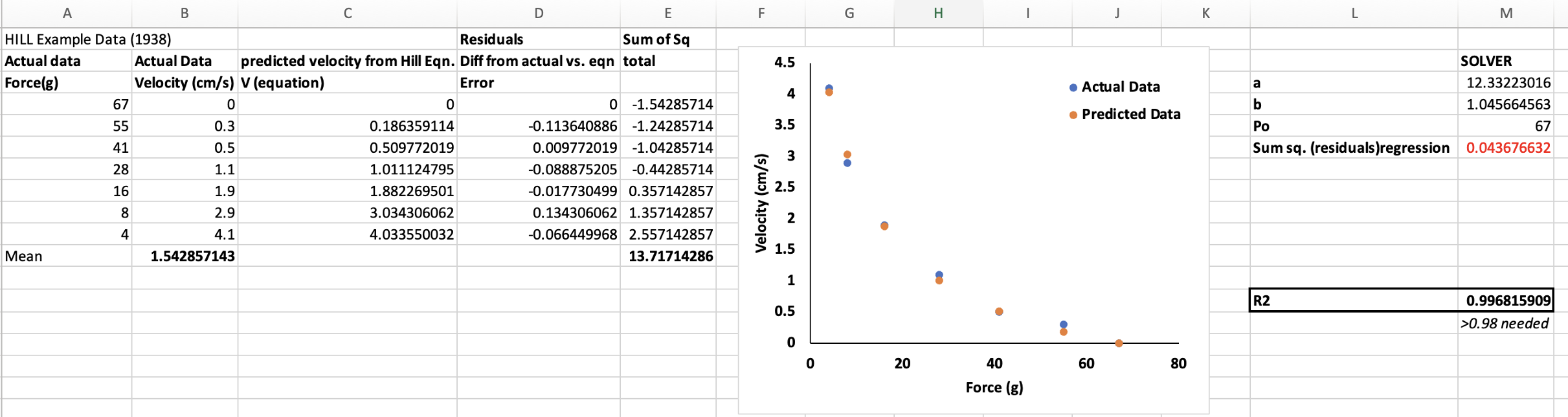 This Solver has ultimately given us values to fill in our original Hill (1938) equation: V = (((67 + 12.33223) 1.04566) / (P + 12.33223)) – 1.04566 From this, we can calculate velocity across an infinite number of force data points, and end up with a very clean force-velocity curve. 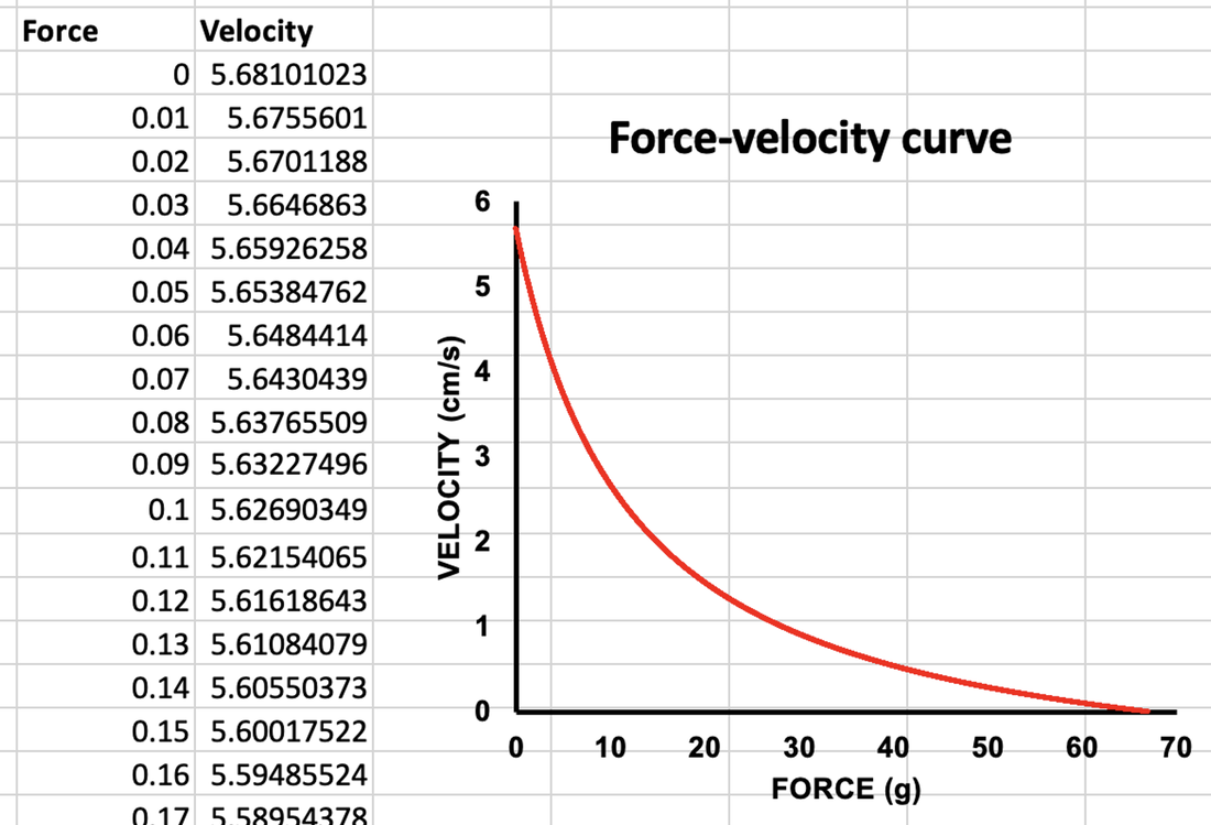 Plotting the data like this also allows us to obtain other key values associated with the force-velocity relationship. For example: the curvature of the force-velocity curve, which is equal to a divided by Po; and the maximum shortening velocity (Vmax), which is nearly impossible to obtain from real data collection. 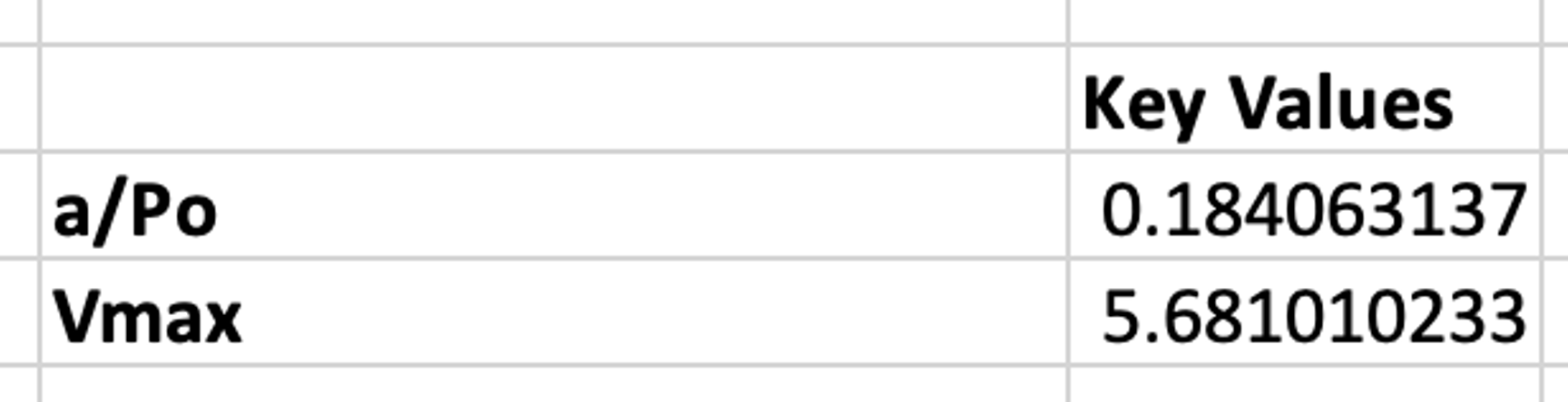 One of the best markers of dynamic muscle performance is power. Power is the product of force and velocity; therefore, we can obtain the maximum power (Pmax) from these data as well. 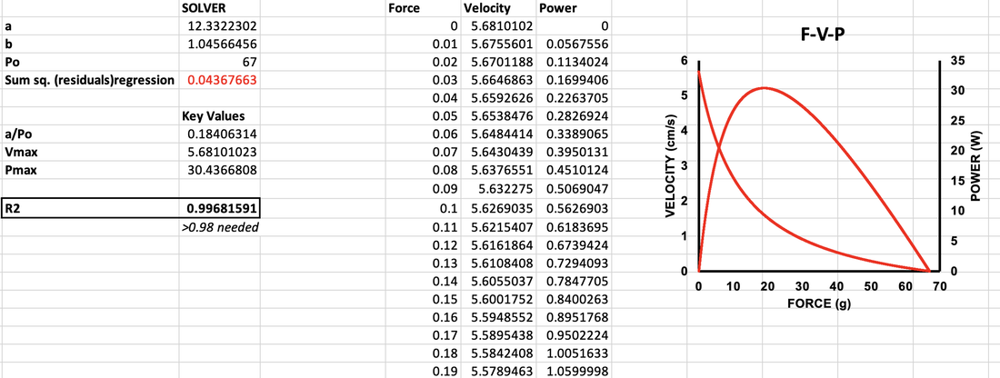 If this process is completed for each participant (whether the data is from a human performing voluntary contractions or a dissected mouse muscle), we can statistically compare the constants and these key values between different groups! For example, the study that produced the graph below compared the force-velocity relationship before (Pre) and after (Post) resistance training, and after a period of de-training (Post-Detr). 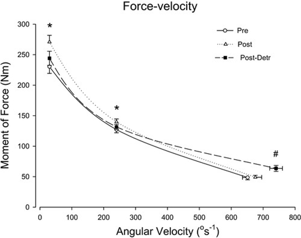 From Andersen et al. (2005), Journal of Applied Physiology. This curve-fitting method works for any equation, including equations with more constants than the force-velocity example I showed here. For example, in a paper by Mohammed and Hou (2015), they suggest using the following asymmetric Gaussian function for fitting the active force-length relationship: 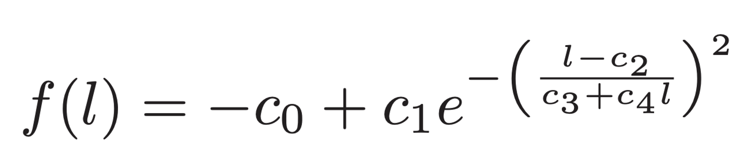 This equation has five constants to adjust for fitting a curve. I have previously used the Excel Solver add-on to fit active force-length data to this equation (see: Hinks et al., 2022, Biology Open), and it worked! Are there any disadvantages to curve-fitting?There are of course limitations to curve-fitting data. The most notable limitation is the accuracy of the equation you wish to use. Staying on the topic of the force-velocity curve, it has long been argued whether this relationship should be represented by a hyperbolic function (the equation used in my Excel example above) or a double-hyperbolic function, which is more intricate: 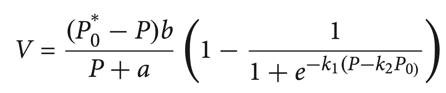 In 1976, Edman and colleagues challenged Hill’s original equation due to various observations over the years where force-velocity data could not be estimated by Hill’s equation. Edman’s findings argued that above 78% of maximum force, there is an inflection point. This inflection point appears to represent a transition toward the shape of the eccentric force-velocity relationship. For the eccentric force-velocity relationship, force is measured during lengthening (as opposed to concentric/shortening) contractions, and an increase in force with increasing lengthening velocity is observed. 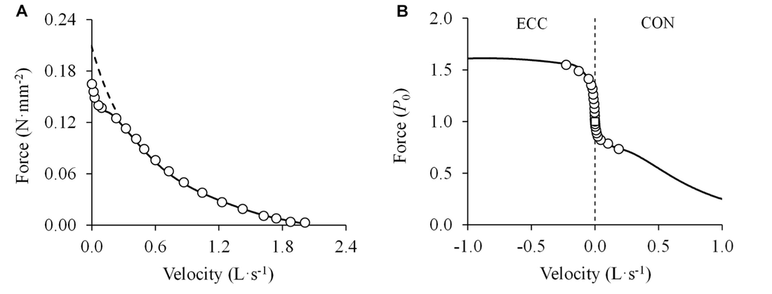 From Alcazar et al. (2019), Frontiers of Physiology. ‘A’ shows a double-hyperbolic force-velocity relationship collected from Edman’s experiments. ‘B’ demonstrates how this double-hyperbolic shape aligns with the shape of the eccentric (ECC) force-velocity relationship. Whether you should employ Hill’s hyperbolic equation or Edman’s double-hyperbolic equation in your curve-fitting is up for debate, and depends on the nature of your experiments. For example, if your experiment incorporates assessment of both shortening and lengthening contractions, Edman’s method is likely better. Alternatively, if your experiment only involves shortening contractions, you could fit your data to both equations and see which produces greater R^2 values. For a more in-depth comparison between these two representations of the force-velocity relationship, look to the review in Frontiers of Physiology by Alcazar and colleagues (2019). Another potential disadvantage to curve-fitting is for some participants, you may end up with a less than ideal R^2 value (for example, 0.90). Here, you may have to decide whether or not to cut said data from your analyses, or at least determine criteria for the lowest R^2 value you will accept. Regardless, curve-fitting is an excellent method of seeing how your data stands among previous literature. For anyone interested, I have provided the Excel sheet for the force-velocity example presented here. If you’ve made it to the end of this knowledge translation piece, I wish you the best in your future curve-fitting endeavours!
References
Alcazar J, Csapo R, Ara I, Alegre LM. On the Shape of the Force-Velocity Relationship in Skeletal Muscles: The Linear, the Hyperbolic, and the Double-Hyperbolic. Front Physiol. 2019 Jun 19;10:769. doi: 10.3389/fphys.2019.00769. PMID: 31275173; PMCID: PMC6593051. Andersen LL, Andersen JL, Magnusson SP, Suetta C, Madsen JL, Christensen LR, Aagaard P. Changes in the human muscle force-velocity relationship in response to resistance training and subsequent detraining. J Appl Physiol (1985). 2005 Jul;99(1):87-94. doi: 10.1152/japplphysiol.00091.2005. Epub 2005 Feb 24. PMID: 15731398. Edman KA, Mulieri LA, Scubon-Mulieri B. Non-hyperbolic force-velocity relationship in single muscle fibres. Acta Physiol Scand. 1976 Oct;98(2):143-56. doi: 10.1111/j.1748-1716.1976.tb00234.x. PMID: 1086583. Hill, A. V. (1938). The heat of shortening and the dynamic constants of muscle. Proceedings of the Royal Society of London. Series B-Biological Sciences, 126(843), 136-195. Hinks A, Jacob K, Mashouri P, Medak KD, Franchi MV, Wright DC, Brown SHM, Power GA. Influence of weighted downhill running training on serial sarcomere number and work loop performance in the rat soleus. Biol Open. 2022 Jul 15;11(7):bio059491. doi: 10.1242/bio.059491. Epub 2022 Jul 25. PMID: 35876382; PMCID: PMC9346294. Knudson, D. (2006). The biomechanics of stretching. Journal of Exercise Science and Physiotherapy, 2, 3-12. Mohammed GA, Hou M. Optimization of Active Muscle Force-Length Models Using Least Squares Curve Fitting. IEEE Trans Biomed Eng. 2016 Mar;63(3):630-5. doi: 10.1109/TBME.2015.2467169. Epub 2015 Aug 11. PMID: 26276984. Zhang X, Liu ZQ, Campbell KS, Wenk JF. Evaluation of a Novel Finite Element Model of Active Contraction in the Heart. Front Physiol. 2018 Apr 23;9:425. doi: 10.3389/fphys.2018.00425. PMID: 29740338; PMCID: PMC5924776. By Avery Hinks Muscles can perform 3 types of contractions: isometric, concentric, and eccentric. In isometric contractions, muscles contract without moving the joint, like when planking. In concentric contractions muscles shorten while contracting, like when lifting a box off the floor. In eccentric contractions, muscles lengthen while contracting, like when lowering a box from a high shelf.  These different contraction types contribute to the properties of muscle called residual force depression and residual force enhancement. What are residual force depression and residual force enhancement?In a previous knowledge translation, I outlined the mechanisms and relevance of residual force depression and residual force enhancement. Following a concentric contraction, muscles are weaker, require more activation from the brain, and feel more effortful compared to an isometric contraction at the same muscle length. This is called residual force depression. Conversely, following an eccentric contraction, muscles are stronger, require less activation, and feel less effortful. This is called residual force enhancement.  Residual force enhancement following an eccentric contraction and residual force depression following a concentric contraction. Adapted from Chen et al. (2020), Journal of Experimental Biology. Essentially, residual force depression makes your muscles less efficient while residual force enhancement makes your muscles more efficient. The mechanisms behind these phenomena come from the cellular level of muscle, in tiny force-producing structures called sarcomeres. Therefore, force depression and force enhancement are as fundamental to muscle as more basic properties like strength and speed. Because they are fundamental, there has been interest in recent years regarding whether force depression and force enhancement are modifiable with training.  Hypothetically, if we can train a muscle to reduce force depression and increase force enhancement, we can make the muscle more efficient! This may be applicable in sport settings or in elderly populations, where small alterations to the efficiency of movement make a big difference.  How can we target residual force depression and residual force enhancement in training?Based on what we know mechanistically about residual force depression and enhancement, we can point to two specific ways to target them in training. First, there is a structural component. Muscle structure is arranged in a hierarchy, with many sarcomere units comprising a muscle fibre, many muscle fibres comprising what’s called a muscle “fascicle”, and many muscle fascicles comprising a whole muscle. Training—particularly resistance training—can have profound effects on muscle structure across this hierarchy.  Because the mechanisms behind residual force depression and enhancement occur in the sarcomere, it is reasonable to believe that adaptations in muscle structure following training may modify residual force depression and enhancement.  The second target for modifying residual force depression and enhancement is the neural component. As mentioned, residual force depression and residual force enhancement are associated with greater and less required activation from the brain, respectively. On top of this, “neural inhibition”, which is when the brain inhibits a muscle’s activity, occurs during residual force enhancement-type contractions. Partly due to this neural inhibition, ~20% of people show no force enhancement at all! We call these people “non-responders.”  Profound neural adaptations occur following training as well. Altogether, we may be able to reduce force depression and improve force enhancement through structural adaptations, neural adaptations, or both. So…can we modify residual force depression and residual force enhancement through training?Unfortunately, not as easily as we would expect based on everything described above. The first investigation into this question came from outside our lab, in a study by Siebert and colleagues. They compared residual force enhancement during leg extension movements (pushing at the hip and knee) between weightlifters and a non-weightlifting reference group.  They observed no statistically significant differences in force enhancement between weightlifters and non-weightlifters. However, as shown by the graph below, when holding the isometric contraction for longer (“t3” in the graph), weightlifters began to show greater force enhancement than the reference group. Therefore, weightlifting showed potential to improve force enhancement, however, not enough to produce a very noticeable difference compared to non-weightlifters.  Figure from Siebert et al. (2016), Journal of Biomechanics. t1, t2, and t3 refer to times further into the isometric contraction following muscle lengthening. Since this initial investigation, our lab has conducted three training studies to obtain a closer look. Each of our first two studies employed two different training programs: one emphasizing eccentric contractions, and one emphasizing concentric contractions. The distinction between these two training types is eccentric training can increase muscle size by making the muscle longer, while concentric training can increase muscle size by making it wider. Therefore, the purpose of these training studies was to target the structural component of force depression and force enhancement. 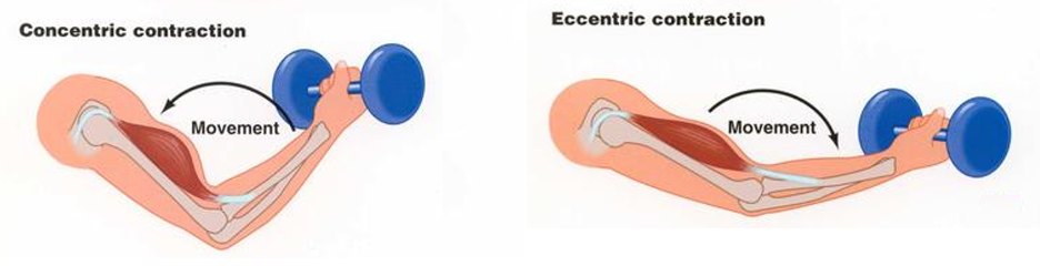 In our first eccentric vs. concentric training study, Chen and Power recruited human participants and submitted them to 4 weeks of training. They observed a 36% decrease in residual force enhancement following eccentric training and an 89% increase following concentric training. So, good, right? Not quite. It appeared that neural adaptations, rather than the targeted structural adaptations, contributed to these alterations to residual force enhancement, mainly by reducing the number of “non-responders” following concentric training. 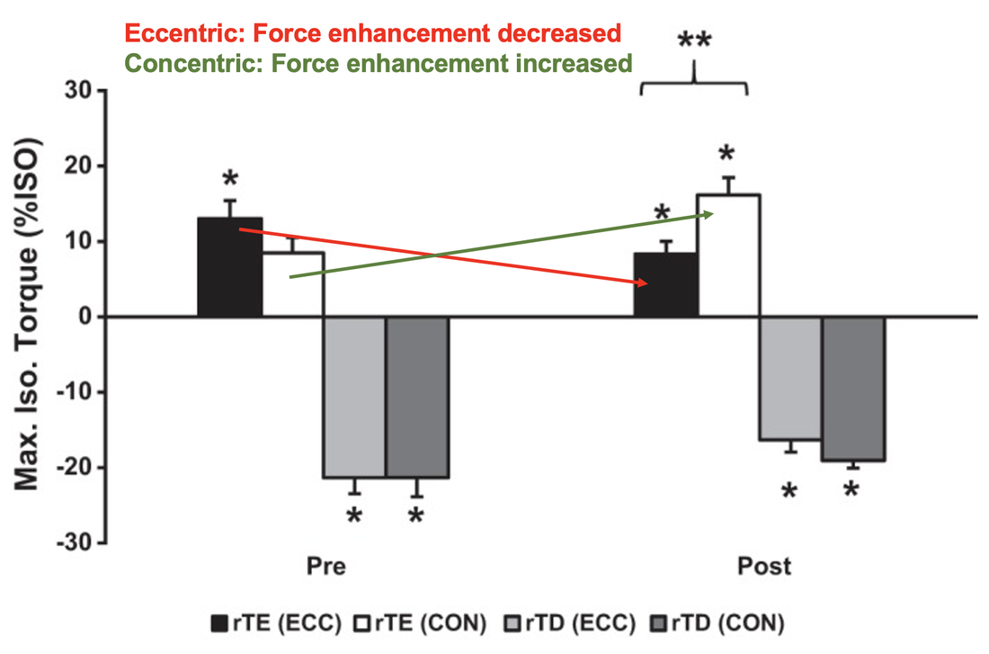 Figure adapted from Chen and Power (2019), Journal of Applied Physiology. Additionally, Chen and Power did not see any alterations to residual force depression following either concentric of eccentric training. This suggests force depression is not modifiable by either structural or neural adaptations to training. Chen and colleagues then went on to perform an eccentric vs. concentric training study in rats. They did this by employing downhill running (which emphasizes eccentric contractions) and uphill running (which emphasizes concentric contractions) training. Testing rats allows us to assess force depression and enhancement in a single dissected muscle, thereby removing the neural components and isolating the structural components of muscle function.  Picture from: https://www.ub.edu/web/ub/en/menu_eines/noticies/2019/07/033.html Consistent with results from the previous human eccentric vs. concentric training study, neither downhill nor uphill running training altered force enhancement or force depression in the muscles of these rats. Additionally, an investigation by Mashouri and colleagues in these same rats showed the same lack of effects on force depression at an even smaller scale, in single muscle fibres. 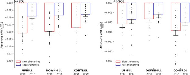 Figure from Mashouri et al. (2020), Physiological Reports. EDL = extensor digitorum longus muscle fibres; SOL = soleus muscle fibres; rFD = residual force depression. Despite these findings showing little influence of muscle structural adaptations on residual force depression and residual force enhancement, we attempted once more to modify these properties through training. In humans, Hinks and colleagues employed isometric resistance training at long and short muscle lengths. Like eccentric vs. concentric training, these training programs are intended to induce different adaptations in muscle structure. Isometric training at a long muscle length may increase muscle size primarily by elongating the muscle, while isometric training at a short muscle length may increase muscle size primarily by widening the muscle.  While we observed the intended adaptations in muscle structure, these did not appear to have any impact on residual force depression or enhancement, as neither changed with training. There was also considerable variability between participants, particularly in how some force enhancement “non-responders” showed force enhancement following training, while others only became “non-responders” after training (as shown in “B” in the graph below).  Figure from Hinks et al. (2021), Scandinavian Journal of Medicine and Science in Sports. Notice how in B some participants are only non-responders for residual force enhancement (rFE) pre-training, while others are only non-responders post-training. rFD = residual force depression. Current consensus on residual force depression and enhancement with training Currently, the only direct evidence that training may improve force enhancement is following concentric resistance training, due to neural adaptations. Structural adaptations do not appear to alter either force enhancement or force depression, and force depression does not appear to be modifiable with training.  In the human studies, however, we must consider whether measurements of residual force enhancement and residual force depression are reliable from day to day. If they are not reliable, that would, of course, impact the accuracy of our human training study findings. This is a question a study from our lab is currently looking into, and will have to wait for another day!
By Avery Hinks An eccentric muscle contraction is when a muscle stretches while producing force. That can be hard to picture, so think of an eccentric contraction as the lowering phase after lifting something. Whether you are lifting weights at the gym, lifting grocery bags out of your car, or lifting your toddler who is tired and doesn’t want to walk anymore, there will come a time when you need to lower what you’ve lifted.  You don’t want to simply let what you’ve lifted drop to the ground (especially if it’s your toddler), so you control the lowering motion. To have this control, your muscles are contracting while stretching. This is an eccentric contraction!  Eccentric contractions are much more than just controlling the lowering of a weight, however. They also demonstrate one of the best examples of the extreme and rapid adaptability of the body’s muscular system. Muscle damage induced by eccentric exerciseWhat if instead of one eccentric contraction, you do 100 or more eccentric contractions? In the lab, we have equipment that allows us to isolate such exercise, but in the real world this might occur in a long downhill hike or a very intense gym session.  A muscle’s strength comes from force produced by the smallest structural units within the muscle, called “sarcomeres.” When your muscle stretches while contracting, sarcomeres stretch too. If sarcomeres repeatedly stretch while producing force, they break apart. This damage has profound effects on the muscle as a whole.  These effects include muscle weakness that can last a whole week, and an inflammatory response that causes intense muscle soreness. The graphs below are classic representations of these impairments. The top graph shows the strength generated in a maximal-effort contraction in arm muscles. Immediately following intense eccentric exercise (“Post” on the graph), strength was reduced by 40%, and remained below the pre-exercise strength value for at least 5 days. As shown by the bottom graph, alongside this prolonged loss of strength, the muscle also experienced soreness 1 to 4 days following the exercise. 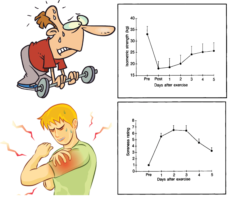 Graphs adapted from Clarkson and Tremblay (1988), Journal of Applied Physiology While uncomfortable, these effects are not necessarily bad. The muscle is a remarkable thing, and can not only recover, but recover stronger! The “Repeated Bout Effect” of eccentric exerciseAs described above, following 1 bout of intense eccentric exercise, the muscle experiences damage and weakness. The response is different, though, following a second, identical bout of eccentric exercise performed 4 weeks later. After the initial exercise bout, adaptations occur in the muscle that protect it from damage during the second bout. Hence the name for this phenomenon: “the Repeated Bout Effect”. The adaptations are widespread, occurring in the brain, the inflammatory system, the connective tissue surrounding the muscle, and the muscle itself. 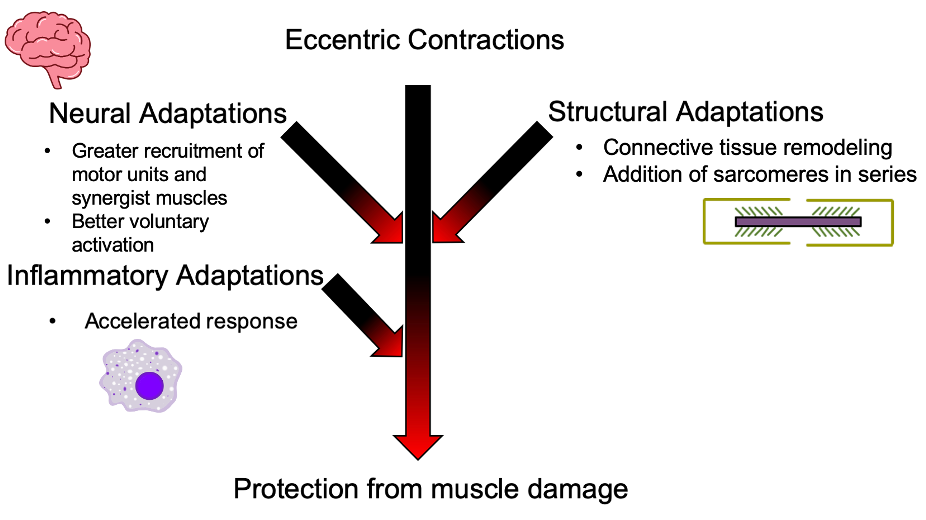 Adapted from thesis by Hess (2017), University of Guelph But what does this really look like? The graphs below are taken from a study in our lab by Hinks and colleagues. Graph A shows the blood levels of an enzyme called Creatine Kinase. Creatine Kinase is an enzyme involved in muscle activity. When sarcomeres are damaged during eccentric exercise, the enzyme leaks out of the muscle fibre cell, eventually ending up in the blood. You can see that following the first bout (black in the graph), a large Creatine Kinase spike occurred. Following the second bout (red), however, Creatine Kinase almost didn’t increase at all, because there was less damage to the muscle’s sarcomeres. 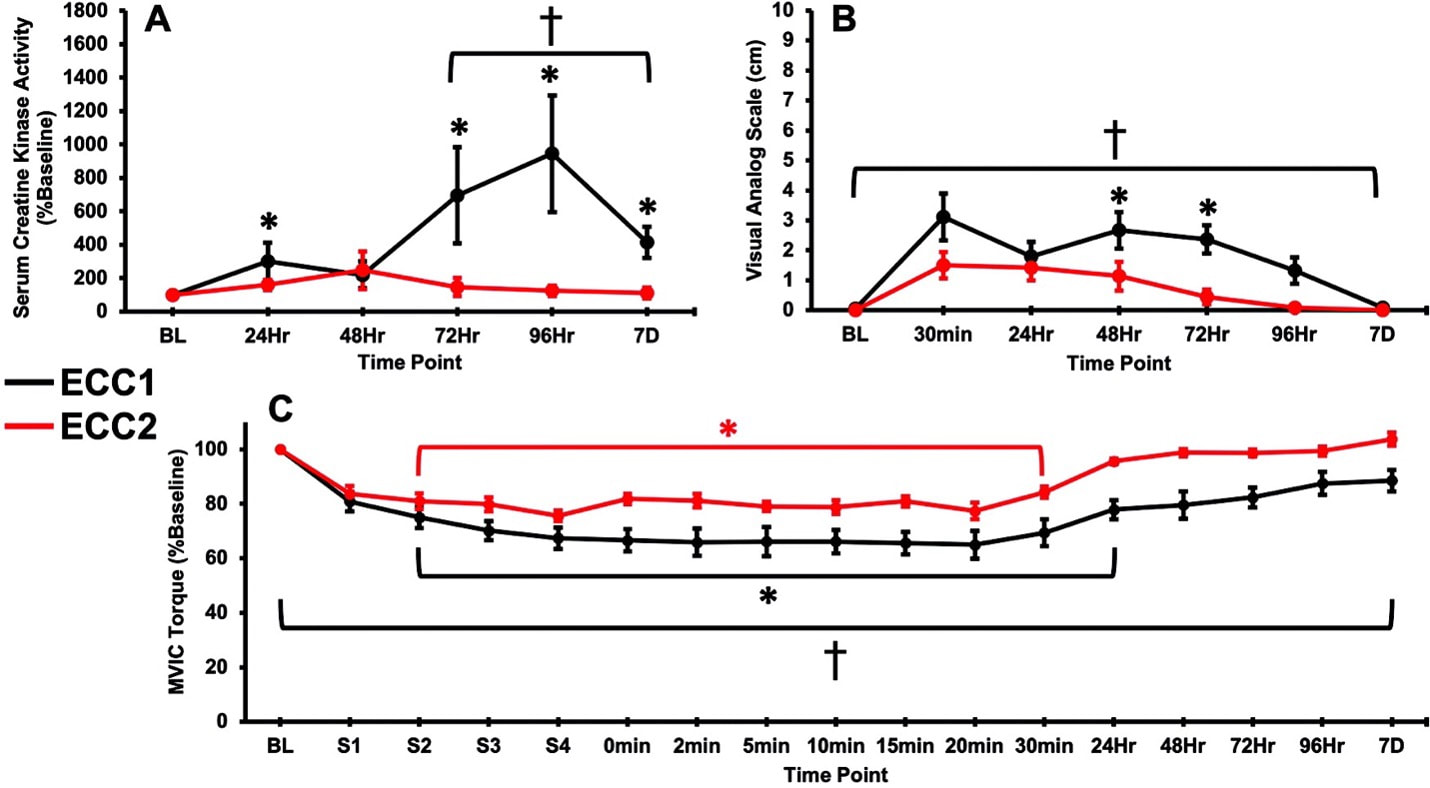 From Hinks et al. (2020), Applied Physiology, Nutrition, and Metabolism The other two graphs show the measures discussed earlier: muscle soreness (B) and maximum strength (C). Graph B shows a clear reduction in soreness in the second (red) compared to the first (black) bout, indicating a reduced inflammatory response. Most importantly, C shows that the muscle experienced less of an impairment in strength immediately following exercise (the “0min” time point on the graph). On top of that, the muscle’s strength recovered earlier, returning to normal the next day (“24Hr”)! Do the benefits of the repeated bout effect apply to everyday life?The measure of maximum strength discussed so far has limited applicability to everyday movements. Strength was assessed in “isometric” contractions, which entails pulling against a fixed object. While isometric contractions are a valid measure of someone’s strength, it does not tell us much about how a muscle performs when moving through a range of motion.  The study form our lab by Hinks and colleagues set out to fill this gap. To do this, they assessed the arm muscles’ “dynamic” performance following an initial and repeated bout of eccentric exercise. The distinction between this “dynamic” performance and the previous “isometric” performance is that now the participants are pulling against an object that can move. Think of it like the action of lifting a weight as fast and hard as you can.  We assessed three important measures of dynamic performance: peak power, rate of force development, and rate of velocity development. I’ll go through them one by one. When measuring dynamic performance in muscle, two factors must be considered: force (or strength) and velocity (or speed). These factors must be considered together because a muscle’s level of force affects how fast it can contract. As a muscle contracts at increasing speed, the amount of force it can produce decreases, and vice versa. Measuring a muscle’s “power” allows us to assess the best of both these factors, because power is equal to force times velocity. Power is especially important in athletes looking to maximize their dynamic performance, such as sprinters and cyclists.  The relationships between force, velocity, and power are best demonstrated by the graph below. You can see that force (solid line) decreases with increasing velocity, and peak power (dotted line) occurs at moderate levels of both force and velocity. 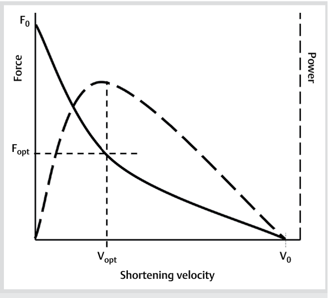 From Jaric (2015), International Journal of Sports Science We can also assess a muscle’s dynamic performance by looking at the rates at which it develops force and velocity. These are called “rate of force development” and “rate of velocity development”, respectively. Rate of force development is exactly as it sounds: a person who reaches maximum force faster will have a greater rate of force development. Rate of velocity development can be more difficult to picture, but it is interchangeable with “acceleration” (yes, like in cars), and describes how fast a person can increase their velocity.  Rate of torque development and rate of velocity development may seem trivial, but they have important applications to everyday life. A prominent example can be found in elderly individuals experiencing falls. If the muscles can react quickly (rate of velocity development) and quickly reach maximum strength (rate of torque development), a fall may be prevented.  We found that the Repeated Bout Effect indeed protects these measures of dynamic performance from muscle damage! In the graphs below, you can see that peak power (A), rate of velocity development (RVD; B), and rate of force development (RTD; C) all experienced less impairment following the second (red) bout of eccentric exercise, and recovered sooner. 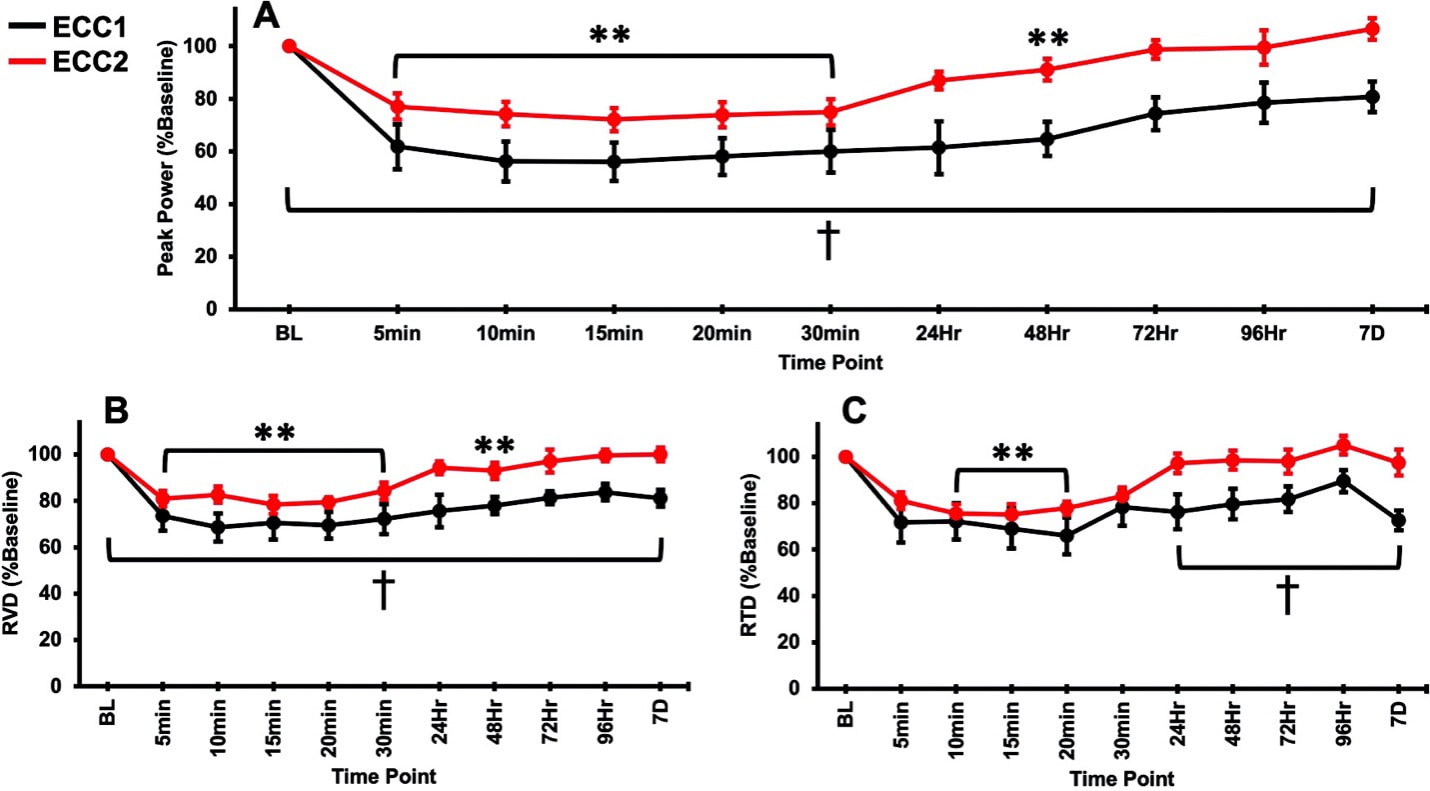 From Hinks et al. (2020), Applied Physiology, Nutrition, and Metabolism What’s the bigger picture?As discussed above, measures of dynamic muscle performance have important real-world applications, such as sport performance and prevention of falls in elderly individuals. Therefore, whether the Repeated Bout Effect’s ability to protect from muscle damage and weakness reduces impairment of these dynamic measures is important—and now we know! This research does not tell the whole story, though. These findings were only determined in arm muscles, while many of the real-world applications discussed apply primarily to leg muscles. Leg muscles do not often display a Repeated Bout Effect as strongly as arm muscles. Therefore, it would be interesting to see whether these dynamic measures are protected in leg muscles as well.  That’s all for now! I hope you’ve learned that the next time your muscles feel sore after a hard workout, that is just your muscles adapting to optimize your performance.
By Avery Hinks Despite what the name might suggest, the “History Dependence of Force” has nothing to do with record-keeping or the superpower used by heroes in Star Wars. Rather, the history dependence of force refers to a fundamental property of how muscles function during movement. Due to its perplexing nature and applicability to real life, it is an often-studied topic in our lab.  To hold the box in this position, the muscles in your arms (mainly the biceps) are undergoing isometric contractions, which means they are sustaining a load (the box) without changing in length. But what if Bob is not there, and you must do all the box-moving alone? Sad, I know. However, depending on whether you are lifting the box from the floor or lowering it from a shelf, your arm muscles might be able make the box easier to carry. Enter the history dependence of force! The definition of the history dependence of force is in the name: it refers to your muscle’s force-producing ability (or its ability to sustain a load, in this case the box) depending on the recent contraction history of that muscle. This “contraction history” can be distinguished into two categories: 1) muscle shortening, or 2) muscle lengthening. Force depression following muscle shortening and force enhancement following muscle lengthening When a muscle shortens to move a load, that is called a concentric contraction. So, let’s say you pick the box up off the floor. In doing this, you must first shorten your arm muscles before assuming an isometric contraction to carry the box out of your house. That prior muscle shortening will hinder your muscle’s force-producing ability, making it harder for you to sustain the isometric load of the box.  This aspect of the history dependence of force is called “residual force depression” and refers to a reduced (or “depressed”) level of isometric force following muscle shortening. In the figure below, you can see that, at the same position following muscle shortening (grey), the level of force the muscle generates is lower than if the muscles are contracting with no prior shortening (black). 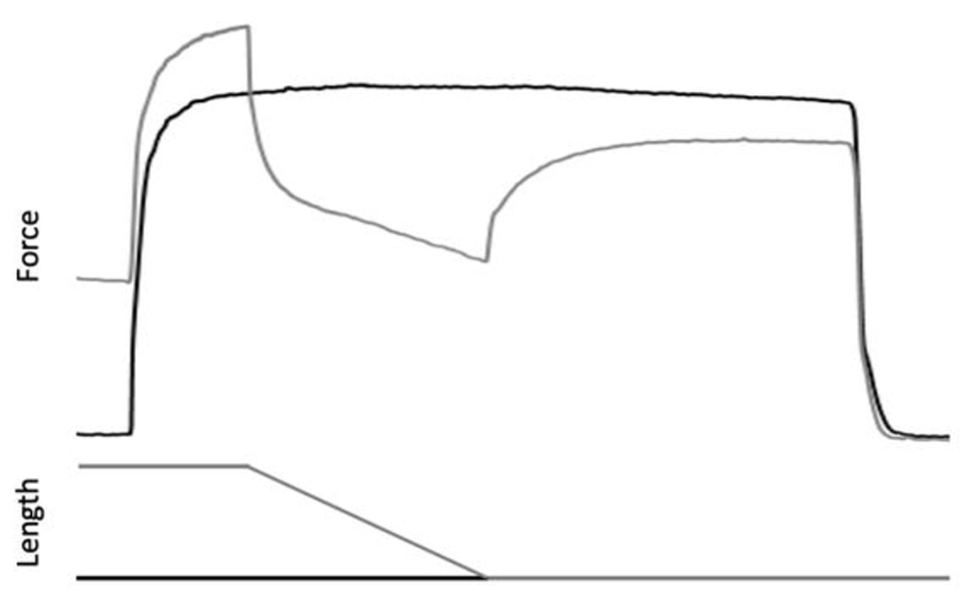 From Chen et al. (2020), Journal of Experimental Biology There’s a flip side, though. What if you lower the box from a high shelf before carrying the box out of your house? Here, your muscles will undergo lengthening while holding the load. We call this an eccentric contraction.  When muscle lengthening precedes an isometric contraction, the muscle can produce more force than it can in a constant isometric contraction. This aspect of the history dependence of force is called “residual force enhancement” because the force is, well, enhanced!  To emphasize with a comparison to the previous figure, you can see below that when an isometric contraction is preceded by muscle lengthening (grey), the muscle’s force is stronger than if an isometric contraction at the same position is not preceded by lengthening (black). 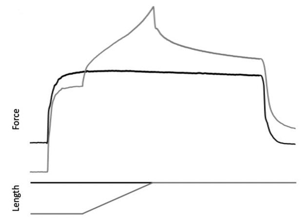 From Chen et al. (2020), Journal of Experimental Biology See, you don’t need Bob! Do force enhancement and force depression impact muscle activity and perception of effort?What do these phenomena of muscle really mean for you? Sure, we can see that our muscles are stronger or weaker depending on whether they are first lengthened or shortened, but can we personally notice if the box feels lighter or heavier? Findings from our lab say yes! The electrical activity of a muscle (measured by a system called EMG) provides insight on the neural input to that muscle, or in other words, how hard the muscle is activating. A study from our lab by Paquin and Power investigated what a muscle’s electrical activity looks like during states of residual force depression and residual force enhancement. They found that, indeed, greater muscle activation is observed in a state of residual force depression, while less activation is observed in a state of residual force enhancement. 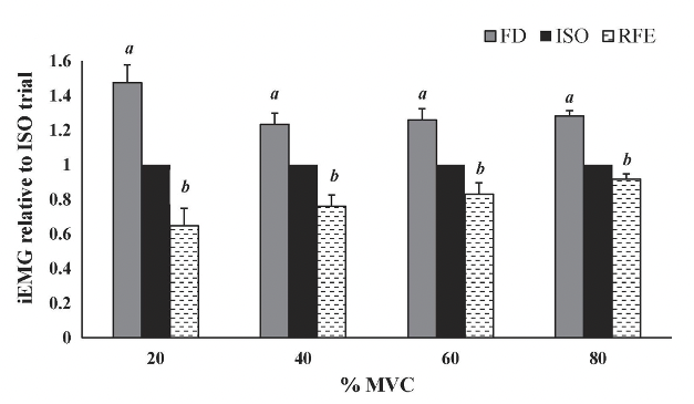 From Paquin and Power (2018), Journal of Electromyography and Kinesiology In the graph above, “%MVC” represents the percentage of maximum muscle strength, and “iEMG” represents the muscle’s electrical activity. It is clear that across all levels of strength, activation is greater during residual force depression (FD in the graph) and less during residual force enhancement (RFE) compared to a regular isometric contraction (ISO). Therefore, we can see that your muscle may requires less input from your brain to hold the box after lowering it from a shelf but may require more input from your brain after lifting the box off the floor.  On top of this, you may also perceive that the box is heavier or lighter. A study from our lab by Kozlowski and colleagues investigated whether perception of effort from a Rating of Perceived Exertion scale (below on the left) differs between states of residual force depression and residual force enhancement. They found that perceived effort was lower in a state of residual force enhancement and higher in a state of residual force depression. 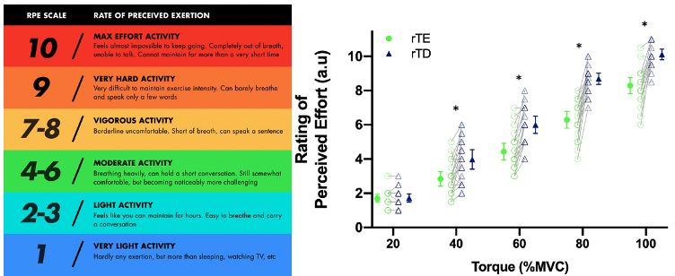 Right is from Kozlowski et al. (2021), Journal of Applied Physiology Like before, in the figure on the right above, “%MVC” represents the percentage of maximal strength. In a state of residual force depression (rTD in the graph, the blue triangles) rating of perceived effort is higher at levels of 40-100% of maximum strength compared to a state of residual force enhancement (rTE, the green circles). Altogether, when you precede an isometric contraction with muscle lengthening, you are stronger, require less muscle activity, and perceive the task to be easier. Conversely, if you precede an isometric contraction with muscle shortening, you are weaker, require more muscle activity, and perceive it to be harder! Why do force depression and force enhancement occur? Even though the history dependence of force was discovered in the 1950s, the mechanisms are still under some debate. The most accepted mechanisms stem from the cellular level of muscle in microscopic units called “sarcomeres”. Sarcomeres generate force in muscle by the formation of “cross-bridges” when proteins called myosin and actin bind together. During muscle shortening, actin becomes deformed, which inhibits formation of some cross-bridges. This inhibition of cross-bridge formation reduces force in the muscle following shortening, leading to residual force depression. In addition to myosin and actin, there is another protein in the sarcomere called titin that acts like a spring when a muscle is stretched.  When a muscle is activated, the length of this spring protein is reduced, increasing the tensile force it produces when stretched. This increase in tensile force from titin leads to greater force in the muscle following lengthening, and thereby residual force enhancement. The bigger picture With these mechanisms behind the history dependence of force in mind, the results on muscle activity and perceived effort in states of force depression and force enhancement make sense:
 Other research from our lab has focused on attempting to modify these properties through training programs. Hypothetically, if we can train a muscle to increase residual force enhancement and decrease residual force depression, we may be able to improve the efficiency of the connection between the brain and muscle during movement. Doing this may have applications in elderly populations, where that connection is often impaired.
That will have to be a topic for another day, though. For now, I hope you’ve learned what the history dependence of force is, and what it might mean for everyday movements. |
AuthorAvery Hinks Archives
September 2023
Categories |
||
 RSS Feed
